OPM: A Compact Deployable Ephemeris Representation for Major Solar-System Bodies with 600-Year Dense Validation

Author: Rz Liu

Abstract

Background. The JPL Development Ephemeris series provides high-accuracy reference ephemerides for Solar-System bodies [1], but complete numerical ephemeris kernels are often impractical for client-side, embedded, or network-distributed applications. A practical deployment route is to transform a reference numerical ephemeris into a compact segmented polynomial representation. Kammeyer (1988) [2], Compressed Planetary and Lunar Ephemerides, is an early and influential engineering implementation of this approach. Modern applications still require a careful balance among file size, random access, runtime cost, and error control.

Objective. This paper introduces OPM, the Orbital Polynomial Model, a compact ephemeris representation for runtime deployment of major Solar-System bodies. OPM is not intended to replace a dynamical integration ephemeris. Its purpose is to provide a small, fast, independently verifiable position-reconstruction model with stable tail-error behavior over a specified coverage interval.

Methods. OPM follows several ideas described by Kammeyer (1988) [2]: remove the dominant orbital structure with body-dependent local coordinates and reference shapes, store Chebyshev residual coefficients, quantize them as integers, and pack the integer coefficients by their actual bit widths in degree-major order. OPM uses a chunked container with per-body model identifiers, sectioned metadata, and explicit residual-coefficient tables. The generation pipeline samples DE441 [1], fits an initial segmented model, and then applies body-specific polishing routes to reduce high-percentile and worst-case errors. The Sun is polished in a native kilometer metric; Mercury, Venus, and the Moon use guarded native-angular polishing; SSB-stored bodies use a heliocentric objective anchored by the already polished Sun model. For validation, DE441 is treated as truth. OPM and Swiss Ephemeris [3] are evaluated on the same Julian-date grid, converted to geometric geocentric J2000 ICRS directions, and compared using angular-error percentiles and maxima.

Results. For a 600-year interval centered near J2000, approximately JD 2378460—2597711 (about 1799-12 to 2400-01, depending on the body-coverage intersection), the validation grid uses the OPM segment structure with 512 Chebyshev nodes per segment plus endpoints, giving 6,810,404 geocentric test samples across the 10 Swiss-addressable major bodies. Across these bodies, the OPM 99th-percentile angular error is at most about 0.00119 arcsec, and 9 of 10 bodies are below 0.001 arcsec. The worst-case error remains below 0.001 arcsec for 7 bodies; Mercury is about 0.00111 arcsec, while Venus and Mars are about 0.00309 and 0.00217 arcsec, respectively. On the same deterministic grid, OPM’s worst-case geocentric angular error is lower than Swiss Ephemeris for all 10 bodies; the largest OPM/Swiss worst-case ratio is about 0.62. A no-expansion ablation shows that body-dependent segment-domain expansion reduces analytic-velocity maximum residuals by about 41%—86% across the Sun, EMB, Mars, Jupiter, Uranus, Neptune, and Pluto. The final 11 OPM files occupy 1.634 MiB in total, or about 278.93 KiB per century.

Conclusions. OPM’s main advantage is bounded-error and tail-accuracy behavior rather than simply minimizing median error. Dense deterministic validation shows that the selected 600-year production instance provides stable high-percentile behavior in a small, randomly accessible representation, and remains below Swiss Ephemeris in worst-case geocentric angular error over this validation grid. The remaining largest tails are the Venus and Mars geocentric composition cases, which motivates future composite-objective polishing and longer-span production validation. OPM is therefore a suitable compact representation for on-demand slicing, distribution, verification, and client-side position queries.

Keywords: ephemerides --- numerical methods --- celestial mechanics --- astrometry --- software: data compression

---

1. Introduction

Modern Solar-System position computation usually relies on high-accuracy numerical ephemerides such as the JPL Development Ephemeris series. DE440/DE441 [1] provide high-accuracy long-span reference data based on dynamical modeling and observational fitting. However, complete kernel files are large, and runtime evaluation normally requires reading and interpreting SPK kernels. This is acceptable for server-side scientific computing, but it is not always the best representation for client applications, network distribution, mobile or embedded environments, or software that needs a fast cold start. In those deployment settings, the more useful object is often a compact, quickly readable, cross-platform, independently verifiable ephemeris representation over a finite coverage interval.

Compact representations of high-accuracy ephemerides have a long history. Kammeyer (1988) [2] described an early complete engineering system in Compressed Planetary and Lunar Ephemerides. Using DE200 as the reference, it compressed the positions of the Sun, Moon, and planets from 1801 to 2049 into a data file of about 830 KB. The system used 40th-degree Chebyshev series, local coordinate axes, reference-orbit subtraction for the inner planets and the Moon, and bit-packed quantized integer coefficients, reporting position errors on the order of 1 milliarcsecond (0.001 arcsec). Kammeyer’s work demonstrated that, for a fixed reference ephemeris and a finite time span, a compact segmented Chebyshev representation can be practical.

OPM adopts the same broad idea: represent a reference numerical ephemeris as segmented Chebyshev series, first remove the dominant orbital structure by local coordinates and reference shapes, then quantize the residual coefficients and pack them by effective bit width. Many engineering choices must still be made explicitly. In this work the reference ephemeris is DE441 [1], and the format adds a modern random-access binary container, CRC checks, body-specific error-polishing targets, and dense deterministic validation focused on worst-case error. Swiss Ephemeris [3] is a mature, widely used compact ephemeris system. It provides small ephemeris files and a unified runtime API for desktop, server, and embedded applications. Therefore, this paper compares OPM with Swiss Ephemeris as a realistic compact-ephemeris baseline, rather than comparing only with the original DE kernels.

OPM, the Orbital Polynomial Model, is a compact binary ephemeris representation for major Solar-System bodies. It is not a new dynamical integration ephemeris; it is a segmented polynomial reconstruction model derived from DE441. OPM stores body positions as piecewise Chebyshev polynomials whose coefficients are quantized and written to random-access binary files. Unlike tests based only on average error or random sampling, the OPM generation pipeline focuses on high-percentile and worst-case error. Tail errors matter for deployable ephemerides because user query times are not sampled from the validation distribution. If localized time intervals contain error spikes, random tests can underestimate the true worst-case behavior.

The validation in this paper uses DE441 as truth and compares OPM with Swiss Ephemeris under the same geometric geocentric J2000 ICRS convention. The tested interval is a 600-year interval centered near J2000, approximately JD 2378460—2597711 (about 1799-12 to 2400-01, with exact endpoints depending on the body-coverage intersection). The validation grid is not random. It is built from the OPM segment structure: 512 Chebyshev nodes per segment plus the segment endpoints. OPM and Swiss Ephemeris are evaluated on exactly the same Julian dates, converted to geocentric vectors, and compared against vectors derived from DE441. The goal is to expose local tail errors, not to estimate an average over a user-query distribution.

Over this 600-year interval the dense validation contains 6,810,404 geocentric test samples across the 10 Swiss-addressable bodies. OPM gives stable sub-milliarcsecond tail accuracy for most major bodies: 9 of the 10 Swiss-addressable bodies have a 99th-percentile geocentric angular error below 0.001 arcsec, and the largest 99th-percentile error is about 0.00119 arcsec. Seven bodies have worst-case errors below 0.001 arcsec. Mercury’s worst-case error is about 0.00111 arcsec, while Venus and Mars are about 0.00309 and 0.00217 arcsec, respectively. On the same validation grid, OPM’s worst-case geocentric angular error is below Swiss Ephemeris for all 10 bodies, with the largest OPM/Swiss worst-case ratio about 0.62.

The rest of the paper is organized as follows. Section 2 describes the OPM segmented Chebyshev representation, coordinate conventions, and binary container. Section 3 describes generation from DE441 and the body-specific error-polishing routes. Section 4 defines the validation convention, including geocentric reconstruction, Swiss Ephemeris flags, and the dense deterministic grid. Section 5 reports the 600-year validation results. Section 6 discusses alternative compression routes that were considered but were not adopted as the main design. Section 7 discusses deployment use cases, the relationship to Swiss Ephemeris and Kammeyer (1988), and current limitations. Section 8 concludes.

---

2. OPM Representation

OPM represents the position of a body over a given time range as Chebyshev polynomials over consecutive segments. An OPM file is a sectioned binary container: a small fixed header identifies the file and section table, while separate sections describe coverage, grid and model parameters, reference-shape data, quantized residual coefficients, metadata, and integrity checks. At runtime, a Julian date selects a segment; the residual coefficients for that segment are dequantized and evaluated, then composed with the body-specific reference model to reconstruct the target position.

2.1 Segmented Chebyshev model

For each segment, OPM maps time from the Julian-date interval [t0, t1] to the standard Chebyshev interval [-1, 1]:

$$u = 2\frac{t-t_0}{t_1-t_0}-1.$$

If a full position vector is represented directly, it can be written as

$$\begin{aligned} \mathbf r(u) &= [x(u), y(u), z(u)],\\ x(u) &= \sum_i a_i T_i(u),\\ y(u) &= \sum_i b_i T_i(u),\\ z(u) &= \sum_i c_i T_i(u), \end{aligned}$$

where T_i is the Chebyshev polynomial of degree i. Chebyshev series provide stable approximation over finite intervals and are convenient for node sampling, error analysis, and tail control. OPM further introduces local coordinates and reference-shape subtraction so that the stored series represents smaller residuals rather than the full position vector.

The formula above describes the nominal runtime segment. The 600-year production instance may fit the polynomial over a slightly expanded domain [t0-Δ_L, t1+Δ_R] while keeping the runtime query interval [t0,t1]. This segment-domain expansion is a generation-time strategy, not a file-format rule; it mainly suppresses analytic-derivative spikes near segment boundaries.

2.2 Local coordinates and reference-shape subtraction

Kammeyer (1988) [2] introduced body-specific coordinate axes before coefficient storage, so that planetary and lunar motion lies close to a local XY plane, and also subtracted reference orbits for the inner planets and the Moon. OPM applies the same principle. Before fitting the residual Chebyshev coefficients, DE441 [1] samples are transformed into body-dependent local coordinates and a reference shape is subtracted.

In local coordinates, the target position can be written as

$$\mathbf r_{\mathrm{local}}(u)=\mathbf r_{\mathrm{ref}}(u)+\delta\mathbf r(u),$$

where r_ref is the reference shape and delta r is the residual vector. OPM primarily stores the Chebyshev coefficients of delta r, not the coefficients of the full position. Because the reference shape absorbs most of the smooth orbital motion, the residual coefficients usually have a much smaller dynamic range. This reduces the size of the quantized integers and the number of bits needed for packing.

Importantly, OPM’s “reference term plus residual term” is first a unified file-representation and read-time idea, not a requirement that all bodies use the same reference-construction method during generation. At runtime, the reader uses the model identifier in the file to obtain the corresponding reference information and quantized residuals, combines them into a Chebyshev representation that can be evaluated for the current segment, and then applies the coordinate convention of that model to recover the global position. Thus the reader sees a uniform set of model identifiers, model parameters, and residual-coefficient payloads; it does not need to know which fitting or search procedure produced those numbers.

Generation can therefore choose different reference-construction routes by body. The first route is direct XYZ fitting: for an object such as the Sun, whose stored vector is already compact enough and does not need an additional local-orbit reference, the generator can directly fit the SSB-to-body XYZ Chebyshev coefficients and then quantize and pack them. The second route is a local-frame shared-reference-shape route: for Mercury, Venus, and most barycentric bodies, the generator transforms samples into a local orbital frame, subtracts a shared reference shape in position space, and fits the remaining residual. The third route is a coefficient-reference route: for the Moon, whose periodic structure is strong but not as well captured by a simple position-space shared shape, the generator first obtains Chebyshev coefficients for each segment on a fixed segment grid, constructs reference coefficients in coefficient space, and stores each segment’s quantized difference from those reference coefficients.

The main difference among these routes is how the reference term is produced, not whether they form completely unrelated runtime systems. Whether the reference term degenerates to an empty reference, comes from a shared shape in position space, or comes from reference coefficients in coefficient space, it is ultimately represented in the OPM container as model parameters and residual payloads and is interpreted by the reader according to the model identifier.

2.3 Body-dependent coordinate conventions

Different bodies use different natural native vectors:

• Sun: Solar-System barycenter (SSB) to Sun;
• Mercury and Venus: heliocentric native vectors;
• Moon: geocentric Earth-to-Moon vector;
• EMB and the outer planets: SSB-to-body or SSB-to-barycenter vectors.

For geocentric comparison, OPM reconstructs Earth and the target body in a consistent way. The Earth is reconstructed from the Earth-Moon barycenter and the lunar vector:

$$\mathbf r_\oplus=\mathbf r_{\mathrm{EMB}}-\frac{\mathbf r_{\mathrm{Moon}}}{1+\mathrm{EMRAT}},$$

with the DE441 value

$$\mathrm{EMRAT}=81.300568221497215.$$

Conversely, when an external EMB reference is needed from an ephemeris interface that provides Earth and Moon but not a direct EMB object, the same relation can be inverted as

$$\mathbf r_{\mathrm{EMB}}=\mathbf r_\oplus+\frac{\mathbf r_{\mathrm{Moon}}}{1+\mathrm{EMRAT}}.$$

2.4 Quantization and binary container

OPM files do not store floating-point Chebyshev coefficients directly. Residual coefficients are divided by fixed quantization steps and rounded to integers. The signed integers are represented with ZigZag coding, then packed by the actual bit width needed for each axis and polynomial degree. In the OPM container, these data are carried by explicit sections: grid and coverage information, model identifiers and parameters, quantization tables, bit-width tables, residual-coefficient payloads, metadata, and CRC-protected integrity fields are separated rather than being treated as one monolithic coefficient array.

OPM uses residual storage, model-specific metadata, and degree-major bit-level coefficient packing. These representation choices are independent of the particular 600-year production instance evaluated below; other time ranges or body subsets can use the same container semantics with different generation parameters.

---

3. Generation and Error Polishing

OPM generation has two phases. The first phase samples DE441 and builds an initial compressible model for each segment. The second phase locally adjusts a small number of quantized integer coefficients, without changing the file structure or bit-width tables, to reduce high-percentile and worst-case errors. The first phase determines the main structure of the model; the second phase mainly handles tail spikes introduced by finite degree and integer quantization.

3.1 Sampling DE441 into segments

The generator is given a target body, a time coverage interval, and a segmentation strategy. The interval is divided into consecutive segments. Within each segment, time is represented by a normalized variable

$$u\in[-1,1].$$

For a segment [t0, t1], the generator samples DE441 at Chebyshev nodes and obtains body positions in the corresponding native coordinate convention. The native convention is the vector representation stored in the file: for example, the Sun uses the SSB-to-Sun vector, Mercury and Venus use heliocentric vectors, the Moon uses the Earth-to-Moon vector, and the outer planets use barycentric vectors.

In terms of initial model construction, the production instance in this paper uses three routes. The first route is direct raw fitting: the Sun’s SSB-to-Sun vector is fitted directly as three-dimensional Chebyshev coefficients, then quantized and polished. The second route is the local-reference-shape route for planets, EMB, and Pluto: the native vector is transformed into a local orbital frame, a shared reference shape is subtracted in position space, and the remaining residual is fitted. The third route is the lunar route: the Moon is also first fitted by raw Chebyshev coefficients on a fixed segment grid, but then a reference coefficient set is subtracted in coefficient space. This can be interpreted as subtracting an equivalent reference for the Moon’s repeated orbital shape in coefficient space.

Segment length, residual degree, reference-shape configuration, and quantization parameters are body-specific. The 600-year data set used in this paper is one production instance; the OPM format itself does not require a fixed epoch, segment length, or body set.

3.2 Local-frame shared reference shapes for planets and Pluto

Except for the Moon, the planets, the Earth-Moon barycenter, and Pluto in the production instance mainly use the same compression route: transform the native vector into a slowly varying local frame, subtract a shared reference shape in that frame, and then fit and store the residual. Here “planets” includes Mercury, Venus, Mars, Jupiter, Saturn, Uranus, Neptune, and Pluto; EMB uses the same class of barycentric-vector route. The Sun’s SSB-to-Sun vector is compact enough to fit directly, so it does not need a separate local reference-shape construction in this section.

The local frame is defined by a unit normal vector and an in-plane angle:

$$\mathbf n=(n_x,n_y,n_z),\qquad \lVert\mathbf n\rVert=1,\qquad \alpha.$$

Here n is the normal vector of the local orbital plane, and alpha is the in-plane periapsis-like direction relative to a reference axis. These are not physical orbital elements; they are numerical compression coordinates. For the planetary, EMB, and Pluto route described in this section, the segment-to-segment normal vector and alpha are not stored as fully independent table values. After estimating the local plane and periapsis-like direction for each segment, the generator represents these slowly varying frame parameters with a first-degree time model over the coverage interval. This first-degree model is a generation-side compression parameterization; it is not a claim that the physical orbit precesses at a strictly constant rate.

During generation, each segment first fits an average plane to the DE441 samples. The smallest-variance direction is taken as the plane normal. Because n and -n describe the same plane, the generator chooses the sign that is continuous with the previous segment. If

$$\mathbf n_s\cdot\mathbf n_{s-1}<0,$$

then the current normal is flipped and the in-plane angle is shifted by half a turn:

$$\mathbf n_s\leftarrow-\mathbf n_s,\qquad \alpha_s\leftarrow\alpha_s+\pi.$$

The geometric plane is unchanged, but the in-plane reference direction remains continuous. The angle alpha is then unwrapped to avoid discontinuities at 2π.

At runtime, the model parameters give (n_x,n_y,n_z) and alpha for the current segment, and the normal is renormalized. A local x/y/z basis is constructed using n as the local z axis. Position samples are projected into this basis and then rotated within the local plane:

$$\begin{aligned} x' &= \cos\alpha\,x+\sin\alpha\,y,\\ y' &=-\sin\alpha\,x+\cos\alpha\,y,\\ z' &=z. \end{aligned}$$

This rotation makes the periapsis-like direction more phase-consistent across segments. The generator then fits a file-wide reference shape in local coordinates. The production route builds the reference shape only for the main in-plane components:

$$\mathbf r_{\mathrm{ref}}(u)=\bigl(S_x(u),S_y(u),0\bigr).$$

Subtracting the reference shape gives the residual samples:

$$\begin{aligned} \delta\mathbf r(u_i) &=\mathbf r_{\mathrm{local}}(u_i)-\mathbf r_{\mathrm{ref}}(u_i)\\ &=\bigl(x'(u_i)-S_x(u_i),\; y'(u_i)-S_y(u_i),\; z'(u_i)\bigr). \end{aligned}$$

OPM fits, quantizes, and packs this residual, not the full position function. Because the local frame and reference shape absorb most of the smooth orbital motion, the residual coefficients usually have a much smaller dynamic range than full raw-coordinate coefficients. This is one of the main reasons that OPM files can be small.

3.3 Direct coefficient models: Sun and Moon

The Sun and Moon do not use the ordinary position-space shared reference shape described above. Their common feature is that the generator first obtains Chebyshev coefficients for the current segment directly, and then proceeds at the coefficient level to quantization, packing, and later error polishing. The difference is that the solar coefficients are already compact enough, while the lunar model further subtracts a reference coefficient set in coefficient space.

The solar route is the simplest one. For the SSB-to-Sun native vector, the generator directly fits three-dimensional Chebyshev coefficients C_s for each segment. These coefficients are not reduced by a local shared reference shape; they enter the subsequent integer quantization and polishing stages directly. In this sense, the Sun can be viewed as a direct coefficient model whose reference term degenerates to an empty reference.

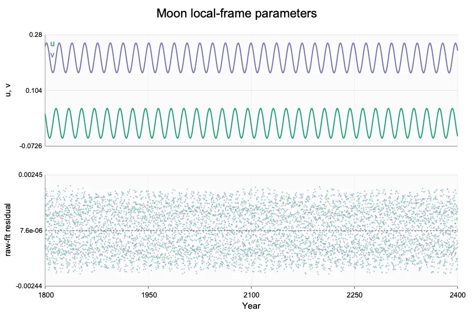
The lunar route adds a coefficient-reference layer on top of the direct coefficient model. The Moon still uses the geocentric lunar vector and a local lunar frame, but the reference term is not a shared S_x(u), S_y(u) curve in position space. It is constructed in coefficient space. This is useful because the Moon has a short period and strong perturbations, so segment-to-segment shape variation is more complex than for planets; subtracting a single shared position-space reference shape does not suppress residuals as stably as in the planetary route. Figure 1 shows the independently fitted per-segment best estimates of the lunar local-frame parameters u and v, together with the affine plus 18.6-year sine/cosine fit actually used by OPM. The scatter already shows a clear periodic structure, which is why the lunar frame parameters are represented by a periodic model rather than by the simpler smooth precession model used in the planetary route.

Figure 1. Lunar local-frame parameters u and v in the fixed-grid coefficient-reference model. Translucent points are independently fitted per-segment best-frame parameters; solid lines are the affine plus 18.6-year sine/cosine fits used by OPM. The two panels show u and v separately; the horizontal axis is calendar year.

Concretely, the lunar route first fits raw Chebyshev coefficients for the geocentric lunar vector on a fixed segment grid, giving a coefficient array C_s for each segment in the local lunar frame. The generator then chooses a reference coefficient set C_ref so that each segment’s difference from that reference is smaller and easier to quantize and pack. The file stores

$$\Delta C_s = C_s-C_{\mathrm{ref}},$$

where s is the segment index. At read time, the quantized ΔC_s is reconstructed and added back to C_ref to obtain the coefficients used for evaluating that segment:

$$\widehat C_s = C_{\mathrm{ref}}+\widehat{\Delta C_s}.$$

Thus the Sun and Moon can both be understood as coefficient routes that first obtain per-segment Chebyshev coefficients. The Sun quantizes those coefficients directly; the Moon first subtracts reference coefficients in coefficient space and then quantizes the differences. Their main distinction from the planetary route is the space in which the reference term is applied: the planetary route subtracts a shared reference shape in position space, the lunar route subtracts reference coefficients in coefficient space, and the solar route does not need an additional reference term.

3.4 Residual Chebyshev fitting and quantization

For each coordinate component, the residual samples are fitted with a finite Chebyshev expansion:

$$\delta r_a(u)\simeq \sum_k c_{a,k}T_k(u),$$

where a is the coordinate axis. To write compact binary files, coefficients are converted to integers using configured quantization steps:

$$n_{a,k}=\mathrm{round}\!\left(\frac{c_{a,k}}{q_k}\right).$$

At read time the stored integer is reconstructed as

$$\hat c_{a,k}=n_{a,k}q_k.$$

The quantization step table is defined by a base step q_base and a degree-dependent multiplier m_k:

$$q_k=q_{\mathrm{base}}m_k,\qquad x_k=\frac{k}{N},$$

where N is the maximum residual degree. The production implementation uses three step modes:

$$\begin{array}{ll} \text{flat:} & m_k=1,\\ \text{growth:}g & m_k=g^{x_k},\\ \text{linear:}a & m_k=1+a x_k. \end{array}$$

Flat steps are useful when coefficient ranges are similar across degrees. Growth steps allow higher-degree coefficients to use slightly coarser quantization, reducing integer magnitudes. Linear steps provide an intermediate option. The q_base values and modes for the production data set are listed in Appendix A.2.

3.5 Bit-width statistics and degree-major bit packing

Quantized coefficients are signed integers. OPM first applies ZigZag coding:

$$\mathrm{zigzag}(n)= \begin{cases} 2n, & n\ge 0,\\ -2n-1, & n<0. \end{cases}$$

Thus 0, -1, 1, -2, 2, … become small unsigned integers. The generator then computes the required bit width for each coordinate axis and polynomial degree. If s is the segment index, the width for axis a and degree k is

$$w_{a,k}=\max_s \mathrm{bit\_length}\!\left(\mathrm{zigzag}(n_{s,a,k})\right).$$

The file stores this axis × degree width table. The payload is written in degree-major order within each axis:

for axis a:
  for degree k:
    for segment s:
      write_bits( zigzag(n[s,a,k]), width = w[a,k] )

This order differs from a conventional segment-major floating-point array. All segments for the same degree are packed together, allowing each degree to use its own minimum safe width.

3.6 Body-specific error-polishing routes

After initial quantization, OPM locally adjusts a small number of integer residual coefficients. This happens only during file generation; runtime readers do not run the optimizer. The polishing step does not change the format, segment structure, or bit-width table. It only tries small ±1 integer modifications around the already quantized coefficients.

Different bodies affect final geocentric direction error in different ways, so OPM uses body-specific objectives:

1. Sun. Solar error directly enters geocentric reconstruction and acts as an anchor for some barycentric-body composite metrics. The Sun is polished in a native kilometer metric.
2. Mercury, Venus, and Moon. These bodies use native-angular guarded worst-case polishing to control their native geometric tail errors directly.
3. EMB, Mars, and outer planets. These bodies are coupled to Earth and the solar anchor in geocentric reconstruction. They are polished with a geocentric composite metric using the already polished Sun model.

This routing avoids applying one scale to all bodies and makes the generation objective closer to the final geocentric viewing-direction error.

3.7 Active and guard grids

The polishing stage is designed to control tail errors rather than RMS or median error. Candidate changes are evaluated on two sets of points: an active grid and a guard grid. The active grid proposes and ranks candidate changes. The guard grid is phase-shifted and is not used to generate candidates; it checks that a candidate does not introduce a new spike at a different phase.

The active grid includes Chebyshev-center nodes, uniform samples, segment endpoints, and endpoint-neighborhood samples. The guard grid uses shifted samples plus endpoint-band nodes. In each local-search round, candidate ±1 integer changes are sorted by a capped lexicographic objective: first reduce peaks above a soft worst-case ceiling, then reduce the actual worst-case error, then improve high-percentile errors. The generator also performs three-point peak refinement near a few local maximum regions to reduce the chance that the true peak lies between discrete samples.

The production route uses:

active grid: Chebyshev-center nodes, uniform samples, and endpoints
guard grid: phase-shifted samples plus endpoint-band nodes
peak refinement regions: 3
objective: capped lexicographic guarded objective
soft worst-case ceiling: 0.00070 arcsec
acceptance: prefer lower worst-case error

The soft ceiling is a generator strategy parameter, not a file-format parameter or a mathematical proof of a global error bound. Final accuracy is reported only from the independent dense validation described in Section 4.

---

4. Validation Design

4.1 Reference truth and comparison system

DE441 [1] is used as the truth source. OPM and Swiss Ephemeris [3] are evaluated at the same Julian dates and compared with DE441-derived geocentric vectors using direction-angle error. The Swiss Ephemeris call used here is swe.calc(), the ephemeris-time interface, not swe.calc_ut(). Therefore the comparison does not introduce a ΔT conversion from universal time to ephemeris time. DE441, OPM, and Swiss Ephemeris all use the same JD values as the ephemeris argument.

Swiss Ephemeris is called through pyswisseph, which is a Python binding to the Swiss Ephemeris C library. The Swiss Ephemeris library version is 2.10.03, the Python binding version is 20230604, and the local C-library source checkout corresponds to official GitHub repository aloistr/swisseph, commit ff04db0 (2026-04-28). The ephemeris files are the official files distributed with the same repository. The flags are:

FLG_SWIEPH | FLG_XYZ | FLG_EQUATORIAL | FLG_J2000 | FLG_TRUEPOS | FLG_ICRS

Swiss Ephemeris returns Cartesian coordinates in astronomical units. This paper uses

1 AU = 149597870.7 km

to convert them to kilometers before comparison.

4.2 Geocentric reconstruction

For each body, DE441, OPM, and Swiss Ephemeris are converted to the same geocentric-vector convention:

$$\mathbf r_{\mathrm{geo}}(\mathrm{body})= \mathbf r_{\mathrm{bary}}(\mathrm{body})-\mathbf r_{\mathrm{bary}}(\oplus).$$

OPM’s internal storage vectors are not all geocentric vectors, so validation composes them according to their storage convention. Earth is reconstructed from the Earth-Moon barycenter and the lunar vector:

$$\mathbf r_\oplus=\mathbf r_{\mathrm{EMB}}- \frac{\mathbf r_{\mathrm{Moon}}}{1+\mathrm{EMRAT}}.$$

The target geocentric vectors are then constructed as

$$\begin{aligned} \mathbf r_{\mathrm{geo}}(\mathrm{Sun}) &=\mathbf r_{\mathrm{Sun}}-\mathbf r_\oplus,\\ \mathbf r_{\mathrm{geo}}(\mathrm{Mercury}) &=\mathbf r_{\mathrm{Sun}}+\mathbf r_{\mathrm{Mercury,helio}}-\mathbf r_\oplus,\\ \mathbf r_{\mathrm{geo}}(\mathrm{Venus}) &=\mathbf r_{\mathrm{Sun}}+\mathbf r_{\mathrm{Venus,helio}}-\mathbf r_\oplus,\\ \mathbf r_{\mathrm{geo}}(\mathrm{Moon}) &=\mathbf r_{\mathrm{Moon}},\\ \mathbf r_{\mathrm{geo}}(\mathrm{body}) &=\mathbf r_{\mathrm{body,SSB}}-\mathbf r_\oplus. \end{aligned}$$

The last line applies to Mars, Jupiter, Saturn, Uranus, Neptune, and Pluto, which are stored as SSB vectors in this data set. Swiss Ephemeris and DE441 outputs are composed to the same geometric geocentric convention before the direction-angle error is computed. This avoids bias from different internal storage conventions.

4.3 Dense deterministic grid

Random sampling can miss short localized tail spikes, especially when error peaks occur near segment boundaries or within Chebyshev oscillations. This paper therefore uses a dense deterministic grid based on the OPM segment structure:

$$512\ \text{Chebyshev nodes per segment}+\text{segment endpoints}.$$

Each body uses the segment boundaries of its corresponding OPM file, restricted to the coverage intersection where OPM, DE441, and Swiss Ephemeris can all be evaluated. OPM and Swiss Ephemeris are evaluated at exactly the same JD grid. The angular error is

$$\mathrm{err}=\mathrm{atan2}\!\left( \lVert\mathbf r_{\mathrm{truth}}\times\mathbf r_{\mathrm{candidate}}\rVert, \mathbf r_{\mathrm{truth}}\cdot\mathbf r_{\mathrm{candidate}} \right),$$

then converted to arcseconds.

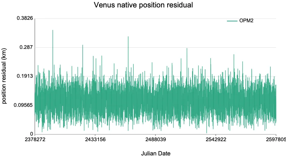
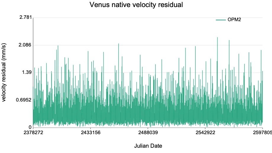
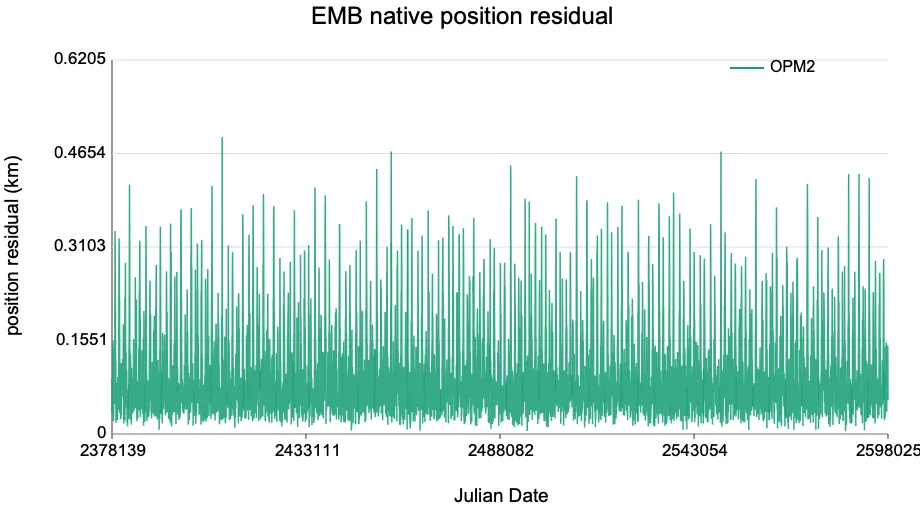
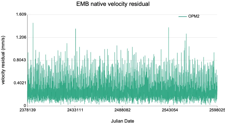
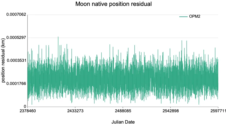
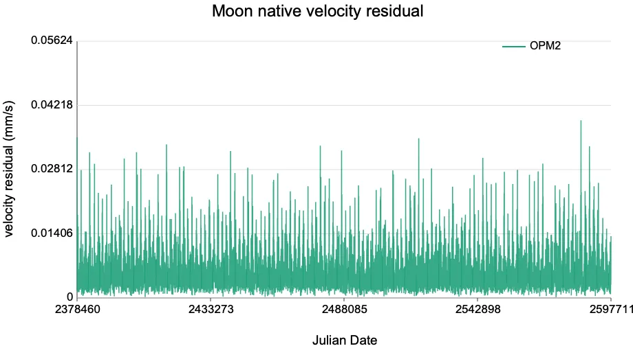
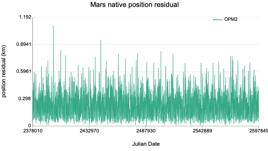
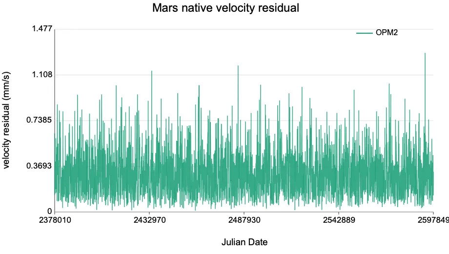
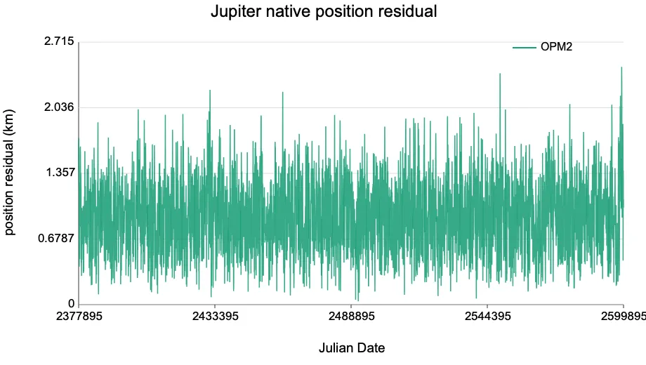
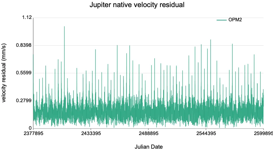
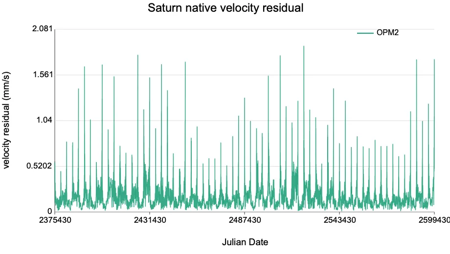
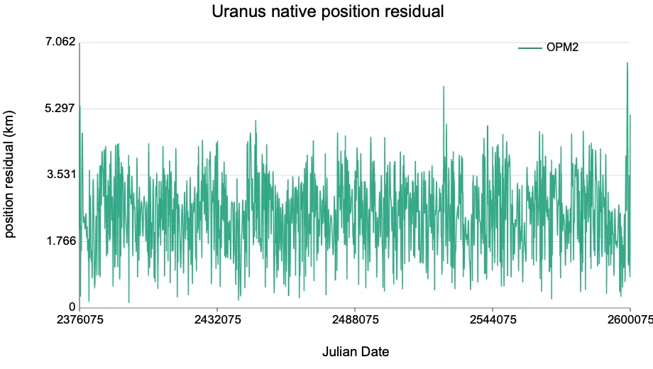
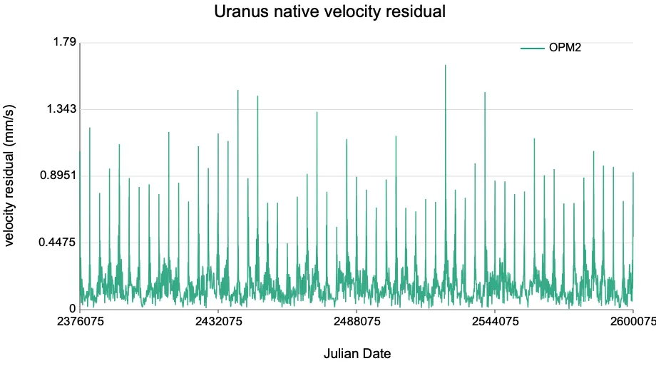
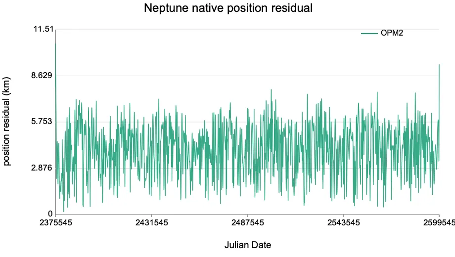
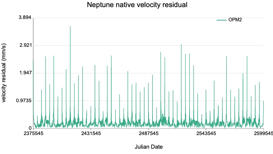
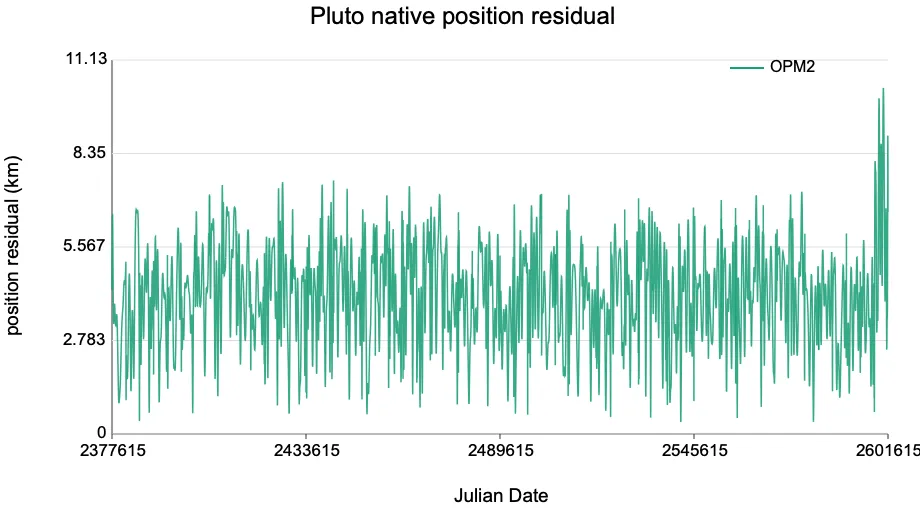
4.4 Native-vector position and velocity residuals

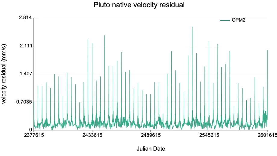
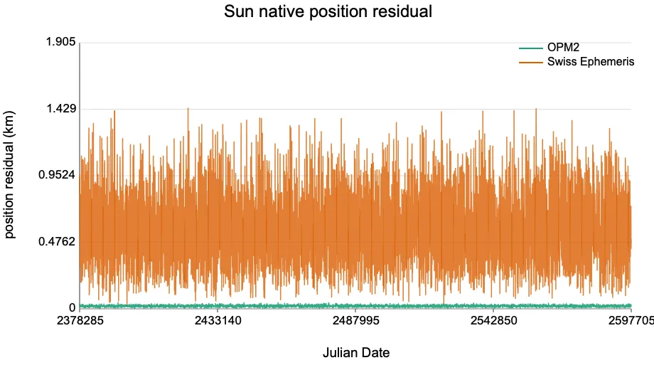
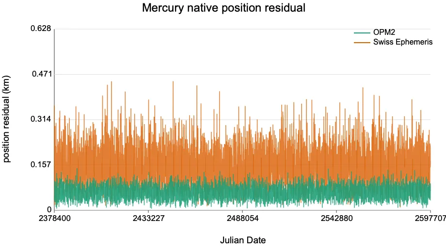
The geocentric angular error is the most direct application-facing metric: it answers how much the apparent direction from Earth differs under a geometric J2000 convention. To enable comparison with the position-residual and velocity-error diagnostics reported by Kammeyer (1988), this paper also computes native storage-vector position and velocity residuals. For each OPM file, the native convention is its stored vector: SSB-to-Sun for the Sun, heliocentric vectors for Mercury and Venus, Earth-to-Moon for the Moon, and SSB-to-body or SSB-to-barycenter vectors for EMB, Mars, Jupiter, Saturn, Uranus, Neptune, and Pluto.

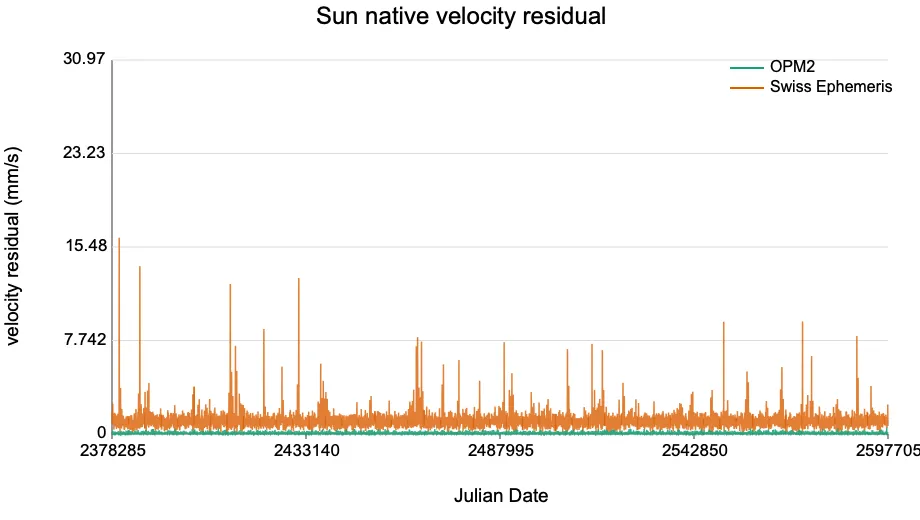
For native-vector comparison with Swiss Ephemeris, the Sun, Mars, and outer planets use barycentric flags; Mercury and Venus use heliocentric flags; and the Moon uses the geocentric lunar vector. Because Swiss Ephemeris does not provide a direct EMB object, the EMB reference is composed from the Swiss Earth SSB state plus the geocentric Moon vector using EMRAT.

The native position residual is

$$\Delta r=\lVert\mathbf r_{\mathrm{OPM,native}}-\mathbf r_{\mathrm{DE441,native}}\rVert,$$

in kilometers. The velocity residual uses the analytic derivative of the OPM Chebyshev representation, not finite differences. If the segment expansion variable is tau and the actual fitting interval is [a,b], then

$$\frac{d\mathbf r}{d\mathrm{JD}}=\frac{d\mathbf r}{d\tau}\frac{2}{b-a}.$$

For bodies using reference terms and local frames, the velocity residual is computed under the file reader’s per-segment fixed-frame semantics: differentiate the reference and residual Chebyshev polynomials, then apply the same per-segment rotation used for position reconstruction. This diagnostic evaluates the analytic velocity continuity and boundary-tail behavior of the compressed representation within segments; it is not an independent dynamical model of the time derivative of frame parameters across segments. DE441 truth velocities are obtained with SPK compute_and_differentiate() in km/day. Reported velocity residuals are converted to mm/s, and the maximum is also retained in AU/day for comparison with Kammeyer’s velocity-error units.

---

5. Results

5.1 Dense comparison with Swiss Ephemeris

Table 1 reports the 512-node dense comparison over the 600-year production coverage, approximately JD 2378460—2597711; exact endpoints differ slightly with the per-body coverage intersections. Errors are in milliarcseconds (mas; 1 mas = 0.001 arcsec). Swiss Ephemeris is used here as a mature compact-ephemeris baseline. The comparison applies only to the geometric geocentric convention, time range, and dense JD grid defined in this paper.

Table 1. Geocentric angular error of OPM and Swiss Ephemeris relative to DE441 on the deterministic dense grid.

Body	Samples	Swiss p50	Swiss p95	Swiss p99	Swiss max	OPM p50	OPM p95	OPM p99	OPM max	max ratio
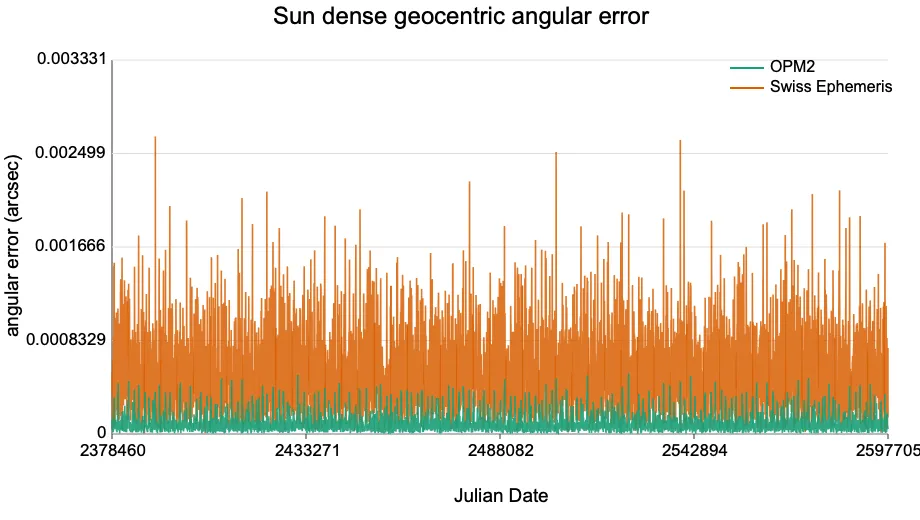
Sun	625,348	0.45303	1.15473	1.5734	3.08471	0.0725509	0.268631	0.394518	0.612202	0.198463
Moon	4,082,040	0.183082	0.381554	0.472806	0.997296	0.088257	0.161144	0.194563	0.354062	0.355022
Mercury	1,279,375	0.481156	1.29911	1.8131	4.01605	0.096465	0.30552	0.479046	1.10924	0.276202
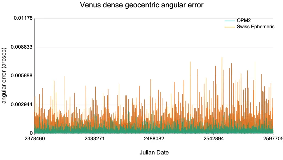
Venus	502,178	0.462357	2.08219	3.94739	10.9045	0.120291	0.633607	1.18861	3.08929	0.283304
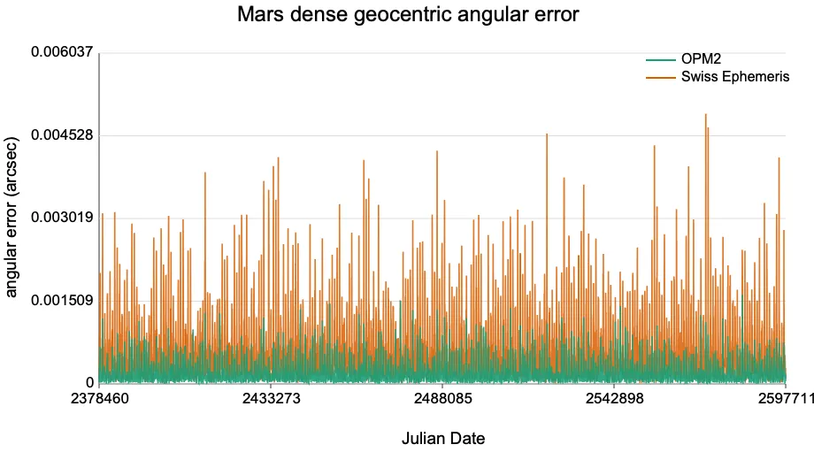
Mars	164,480	0.386527	1.66867	2.70857	5.59026	0.117022	0.544112	0.915997	2.16601	0.387461
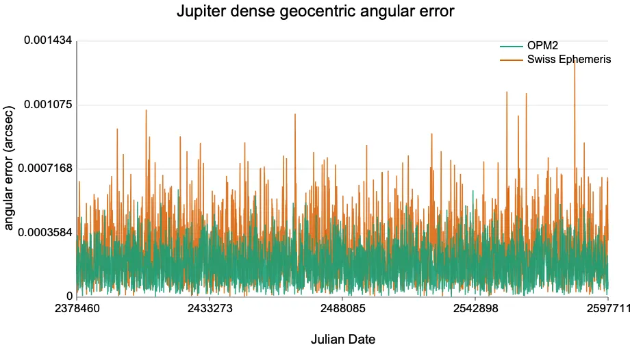
Jupiter	37,963	0.244876	0.580533	0.761804	1.32745	0.16921	0.347107	0.428432	0.62895	0.473803
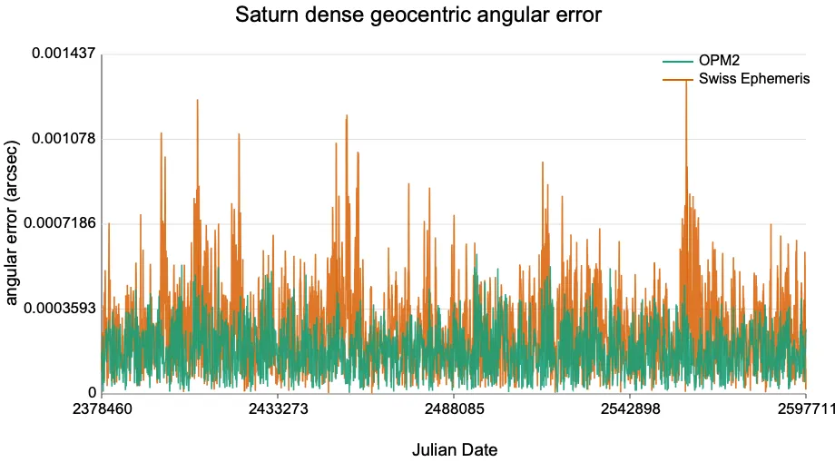
Saturn	32,833	0.246308	0.570078	0.804569	1.33082	0.174783	0.345993	0.426783	0.593456	0.445931
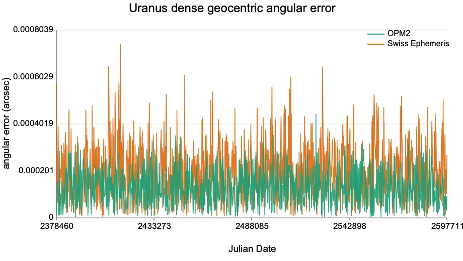
Uranus	28,729	0.181587	0.399819	0.52134	0.744338	0.130098	0.24763	0.290137	0.452878	0.60843
Neptune	28,729	0.175997	0.369308	0.442545	0.56435	0.13576	0.245982	0.278174	0.348089	0.616796
Pluto	28,729	0.17938	0.398675	0.579352	0.902187	0.103139	0.201214	0.255212	0.32977	0.365523

The total number of dense geocentric test samples is 6,810,404.

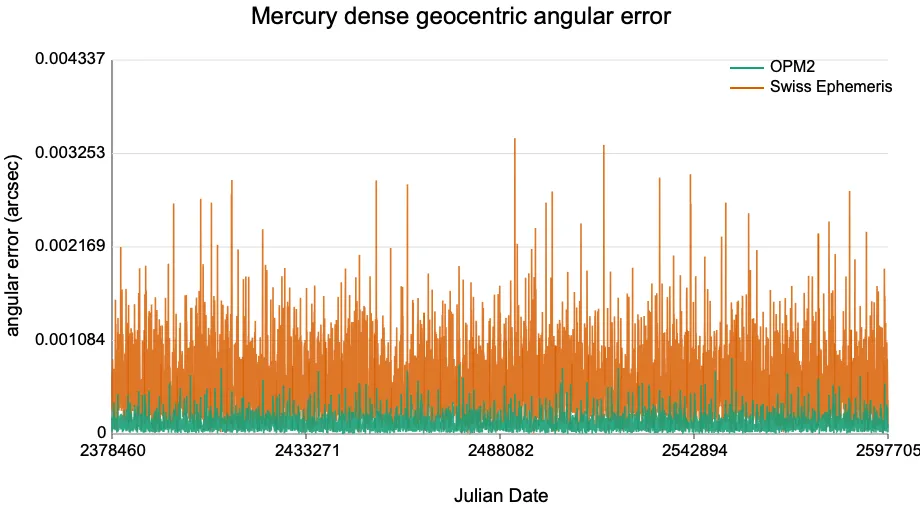
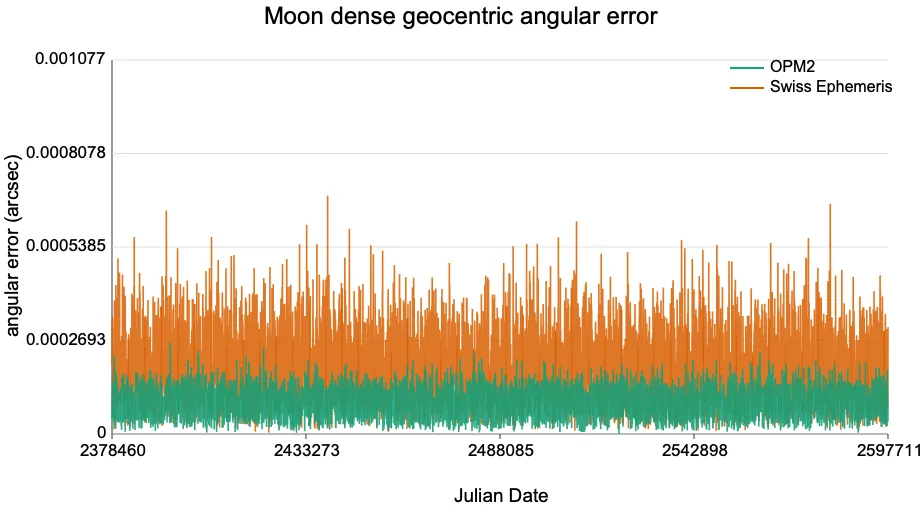
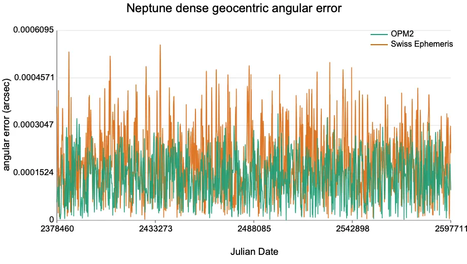
Figure 1 shows representative error curves from the same grid. Mercury represents the short-period, high-eccentricity inner-planet case; the Moon represents the high-segment-count, strongly perturbed case; Neptune represents a long-period outer-planet case. The complete set of 10 SVG curves is listed in Appendix D and is generated from the same run as out/opm2-600y-selected-polished-swiss-geocentric-512.txt.

Figure 1. Representative geocentric angular-error curves on the 600-year dense grid. Green is OPM; orange is Swiss Ephemeris. The vertical axis is arcseconds.

Mercury	Moon	Neptune

5.2 Native-vector position and velocity residuals

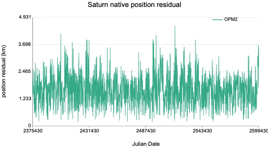
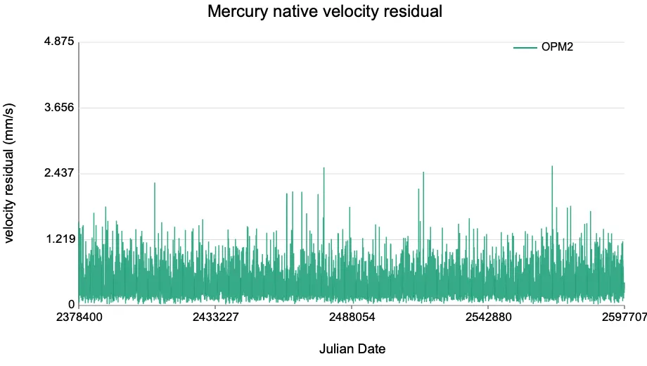
Table 2 gives native-vector residual diagnostics for the same 600-year production instance. This table does not compare with Swiss Ephemeris and does not replace the geocentric angular-error result. It reports OPM’s representation error in the storage-vector convention itself. The velocity columns are analytic-derivative errors and therefore also probe continuity and tail behavior at the derivative level.

Table 2. OPM native storage-vector position and velocity residuals relative to DE441. Position is in km; velocity is in mm/s. The last column converts the velocity maximum to AU/day.

Body	Samples	pos p99	pos max	vel p99	vel max	vel max (AU/day)
Sun	626,566	0.0368692	0.0593164	0.347994	0.579346	3.35e-10
EMB	309,428	0.342282	0.574572	0.861984	1.48942	8.60e-10
Moon	4,089,898	0.000399791	0.000653896	0.0233432	0.0520753	3.01e-11
Mercury	1,281,402	0.116896	0.173573	1.39014	4.51347	2.61e-09
Venus	502,178	0.20927	0.354275	1.40304	2.57493	1.49e-09
Mars	164,480	0.617666	1.10381	0.793572	1.36764	7.90e-10
Jupiter	38,036	1.77459	2.51366	0.654538	1.0368	5.99e-10
Saturn	32,896	3.34507	4.5653	1.2746	1.92681	1.11e-09
Uranus	28,784	4.52432	6.53912	1.03322	1.65757	9.57e-10
Neptune	28,784	6.98715	10.6528	2.02844	3.6056	2.08e-09
Pluto	28,784	7.18292	10.3089	1.69146	2.60561	1.50e-09

Figure 2 gives two representative curves. The Saturn position residual provides a direct analogy with Kammeyer’s Saturn residual figure in kilometers. The Mercury velocity residual shows a derivative-sensitive case for a short-period inner planet. The full native position and velocity residual curves are listed in Appendix E and are generated from the same diagnostic run as out/opm2-600y-selected-polished-native-residuals-512.txt.

Figure 2. Representative native-vector residual curves. Left: Saturn native position residual in km. Right: Mercury native velocity residual in mm/s.

Saturn native position residual	Mercury native velocity residual

5.3 Effect of segment-domain expansion on analytic velocity residuals

Table 3 reports a no-expansion ablation for the bodies where segment-domain expansion is most relevant to analytic velocity behavior. Expansion is not a rule of the OPM file format; it is a body-specific generation strategy. Its main benefit is not monotonic improvement of position residuals. Instead, it moves the runtime query interval endpoints into the interior of the fitting interval, substantially reducing derivative spikes amplified at segment boundaries. The comparison below uses the same selected 600-year raw configuration with expansion enabled versus a regenerated raw configuration with segment_domain_expansion_fraction = 0.0; both are evaluated by the same 512-node native residual diagnostic. The Swiss Ephemeris velocity maximum is included as an unchanged external reference for the same native-vector convention where available; EMB is composed from the Swiss Earth SSB state and the geocentric Moon vector using the DE441 mass ratio.

Table 3. Effect of segment-domain expansion on analytic velocity maxima. Velocity is in mm/s.

Body	selected velocity max	no-expansion velocity max	reduction	Swiss velocity max
Sun	0.526687	2.309811	77.198%	28.673538
EMB	1.268522	8.728240	85.466%	20.603949
Mars	1.210830	8.527175	85.800%	19.486554
Jupiter	0.847487	3.956380	78.579%	5.271369
Uranus	1.303232	5.184090	74.861%	4.720532
Neptune	2.916734	5.517831	47.140%	5.464040
Pluto	2.249976	3.792159	40.668%	7.193522

5.4 Summary by statistic

Table 4 summarizes which system has the lower error for each statistic under this paper’s validation grid and angular-error definition. “Lower” refers only to this specific comparison convention and does not rank the systems as complete software packages.

Table 4. Number of bodies for which each system has the lower error statistic.

Statistic	OPM lower	Swiss Ephemeris lower	Note
p50	10	0	OPM is lower for all listed bodies
p95	10	0	OPM is lower for all listed bodies
p99	10	0	OPM is lower for all listed bodies
max	10	0	OPM is lower for all listed bodies

5.5 Worst-case error ratio

Table 5 gives the ratio of Swiss Ephemeris maximum error to OPM maximum error. A ratio larger than 1 means that, in this validation convention, the Swiss Ephemeris maximum error is larger than the OPM maximum error.

Table 5. Worst-case angular-error ratio relative to OPM.

Body	Swiss Ephemeris max / OPM max
Sun	5.04×
Moon	2.82×
Mercury	3.62×
Venus	3.53×
Mars	2.58×
Jupiter	2.11×
Saturn	2.24×
Uranus	1.64×
Neptune	1.62×
Pluto	2.74×

The percentile results show that the largest differences are in the distribution tails. In the updated 600-year production instance, OPM is lower than Swiss Ephemeris for p50, p95, p99, and maximum error for every listed body. Neptune and Uranus remain among the closest outer-planet cases, but their OPM worst-case errors are still only about 62% and 61% of the Swiss Ephemeris maxima, respectively.

5.6 File size

Table 6 gives the actual OPM file sizes in the 600-year production instance. These sizes are not externally compressed with gzip or similar tools. They include the file header, segment index, reference shape, model tables, quantized residual bitstream, and checksums. The per-century values are the 600-year sizes divided by 6 and should be interpreted only as an average scale.

Table 6. OPM production file sizes for 600 years and per-century equivalents.

Body	600-year size (KiB)	per-century size (KiB/century)
Sun	99.73	16.62
Mercury	182.30	30.38
Venus	86.72	14.45
EMB	75.51	12.59
Moon	1158.91	193.15
Mars	39.82	6.64
Jupiter	9.92	1.65
Saturn	8.16	1.36
Uranus	4.75	0.79
Neptune	3.67	0.61
Pluto	4.10	0.68
Total	1673.60 KiB = 1.634 MiB	278.93

The Moon dominates the current size, accounting for about 69% of the total 600-year data set. Mercury, the Sun, Venus, and EMB follow. The outer planets move more slowly and have fewer segments, so their individual 600-year files range from a few KiB to about 10 KiB. As a same-interval file-size reference, the corresponding core files in the local DE441-based Swiss Ephemeris installation are sepl_18.se1 for the Sun through Pluto and semo_18.se1 for the Moon; together they occupy 1,788,832 bytes, or about 1.71 MiB. The main-asteroid file seas_18.se1 is not included in this comparison. If the total per-century size in Table 6 is linearly extrapolated to the full DE441 time span, JD -3100015—8000016 (about 303.9 Julian centuries), the major-body data set would be about 82.9 MiB. This extrapolation is only an order-of-magnitude comparison; it is not a completed full-DE441 production validation.

---

6. Alternative Compression Routes and Design Tradeoffs

Before converging on the OPM representation used in this paper, several natural compact-ephemeris constructions were tested. Some were useful for short spans, specific bodies, or particular runtime targets. However, when long-term stability, file size, runtime cost, implementation complexity, and worst-case error are considered together, they were less robust than the route used here: reference-shape subtraction, local frames, residual Chebyshev series, and bit-level packing.

6.1 VSOP87 and truncated analytic series

A direct idea is to use an existing analytic ephemeris as a base model and compress the difference between it and DE441/JPL. The Swiss Ephemeris documentation [3], Section 2.1.4, states:

Instead of the positions we store the differences between JPL and the mean orbits of the analytical theory VSOP87. These differences are a lot smaller than the position values, wherefore they require less storage. They are stored in Chebyshew polynomials covering a period of an anomalistic cycle each.

This is an important clue: the compressed object is a residual relative to a mean orbit, not necessarily a full raw position. Interpreting this as “compute the full VSOP87A/VSOP87B position and store JPL minus VSOP87” overstates the role of the full analytic series and exposes several tradeoffs.

In early experiments, VSOP87A plus DE441/JPL residuals reached about the 0.001 arcsec level, and VSOP87B plus residuals could reach about 0.0001 arcsec. But the full VSOP87B series has many terms and is too expensive for a small client-side runtime. Truncating VSOP87 improves speed but leaves long-term phase errors that grow away from the modern epoch. A truncated-VSOP87B plus correction route reached about 0.8” peak error over roughly ±4000 years, but degraded beyond that. More elaborate variants, such as merging nearby frequencies or adding century-level correction layers, improve local behavior but increase format complexity and still leave long-term phase structure in the residual.

The lesson is not that analytic series are inaccurate. Rather, high-accuracy analytic series are too heavy, while strongly truncated series leave residuals that are difficult to compress uniformly over long spans.

6.2 Steve Moshier’s PLAN404 trigonometric reference model

After truncated VSOP87 showed long-term divergence, another attempt used Steve Moshier’s PLAN404 package [4] as a reference model. PLAN404 contains trigonometric series for the planets fitted to JPL DE404 Long, approximately from 3000 BCE to 3000 CE, and outputs heliocentric ecliptic coordinates. The stated raw accuracy ranges from about 0.1” for Earth to about 1” for Pluto.

The purpose of using PLAN404 was not to make it the final ephemeris. It was to test whether a smoother long-term semi-analytic reference could reduce the difficult residual structure left by truncated VSOP87. Internally, raw PLAN404 residuals against DE441 could reach tens of arcseconds over ±5000 years, but the residuals changed more smoothly and could be reduced by low-degree segmented corrections. The main bottleneck was a quasi-periodic term near 40 years whose amplitude grows away from the modern epoch.

PLAN404-like references are valuable because they can absorb smooth long-term phase structure. However, they did not solve the file-size problem. For Mercury, a tuned PLAN404 plus spherical residual route was about 116 KB/century. This was smaller than some earlier routes, but still much larger than the later local-frame and reference-shape design.

6.3 Direct numerical fitting and slow-body exceptions

Another route is to bypass analytic ephemerides and directly fit DE441/JPL position tables. The simplest version stores each body’s three-dimensional position as Chebyshev polynomials over fixed time intervals. This is clean and easy to validate, but it compresses the inner planets and the Moon poorly. Without removing the dominant orbital structure, the Chebyshev coefficients must represent the full elliptical motion, plane variation, and perturbations at once. Low-degree coefficients are large and high-degree coefficients do not fall to very small bit widths.

Experiments with velocity constraints or additional spatial/orbital features did not solve the fundamental entropy problem. If the main orbital motion remains in the residual, the coefficients remain hard to pack.

Direct fitting does work for some slow or low-curvature bodies. Early direct-fit Pluto formats achieved a random-test 99th-percentile error around 0.00047 arcsec with small files. This indicates that the compression strategy should be body-dependent: slow objects can sometimes be fitted directly, while inner planets and the Moon require phase, frame, and reference-shape subtraction.

6.4 Kepler ellipses, orbital elements, and spike patches

Another class of methods starts from low-dimensional orbital models, such as yearly or century-level corrected Kepler ellipses, or fitted time-varying orbital elements, followed by local-coordinate residual compression. These models look physically interpretable but are not automatically good compression coordinates.

Mercury is the clearest counterexample. Experiments fitted semimajor axis, eccentricity, inclination, node longitude, perihelion direction, and mean anomaly over a century, then reconstructed a reference ellipse with Kepler’s equation and stored radial-tangential-normal residuals. Mercury has about 415 perihelion cycles per century, and perturbations introduce strong short-period oscillations in instantaneous elements. Low-degree century-level fits produced large structural errors: semimajor-axis fit errors reached about 431,000 km, mean-anomaly errors about 0.17 rad (roughly 10°), and eccentricity errors about 0.02. The runtime cost was also high because it required multiple Chebyshev evaluations, Kepler iterations, many trigonometric functions, and coordinate rotations.

Special spike patches can reduce isolated residual peaks, but they tend to turn the format into a collection of exceptions. More importantly, many spikes are symptoms of systematic mismatch in reference phase, local frame, or reference shape. Patches are not a substitute for choosing a better compression coordinate.

6.5 Special difficulty of the Moon and Mercury

The Moon and Mercury expose the most difficult parts of the compression problem. Mercury is dominated by short perihelion cycles, high eccentricity, and long-term precession. The Moon has even shorter periods, strong perturbations, and complex node/perigee behavior. Earlier lunar formats used perigee segmentation, node/orbit frames, mixed bit-width quantization, and related strategies, reaching about 0.0011 arcsec random-test p99 error, but lunar data still dominated the total size over 30,000-year scales.

Many specialized lunar routes were tested: physical orbit frames, PCA reference shapes, perigee/apogee alignment, fixed rotations, equinoctial orbital elements, low-bit-width tail coefficients, tolerance scans, degree scans, and sampling-budget scans. These experiments show that the lunar challenge is not only residual degree; it is the joint design of phase, frame, and metadata.

Mercury showed a similar lesson. The effective reference is not a direct fit to instantaneous orbital elements, but a compression reference built around mean perihelion phase and a local plane. The Mercury route used here applies a global perihelion-clock correction, local frame, reference shape, and guarded/refined error polishing. The lunar route uses a fixed segment grid, a local frame, and a coefficient-space reference term: it shares the reader-side idea of “reference term plus residual term” with the planetary route, but constructs the reference after raw Chebyshev fitting in coefficient space.

6.6 Early Kammeyer-like OPM2/OPV2 route

Before the OPM representation used in this paper, the earlier OPM2/OPV2 route was the first unified route whose file size approached the scale of the core Swiss Ephemeris ephemeris files. It already used the main Kammeyer-like ingredients: per-segment local frames, fixed quantization units, mixed bit-width packing, Mercury reference-shape subtraction, and fixed principal-component frames for Pluto or other slow objects. In some early tests, this route gave p99 angular errors of roughly 0.0008—0.0015 arcsec.

Kammeyer’s original system also used segment-domain expansion as a boundary-control strategy. For Mercury, Venus, the Earth—Moon barycenter, Mars, the outer planets, and the Sun, the Chebyshev expansions were fitted on intervals extended by 5% of the segment length on both sides; for the Moon, the expansion interval was identical to the segment. This influenced OPM experiments, but OPM does not adopt the 5% value as a fixed rule. The final production data show that segment-domain expansion is most clearly beneficial for analytic velocity residuals, not monotonically for position error. OPM therefore uses smaller body-dependent expansion fractions and validates them explicitly.

Adaptive segment lengths were also explored. They can be effective for a single body under a single error threshold, but they add segment-boundary metadata, complicate random access, and weaken the regularity of global clocks, shared reference shapes, and degree-major packing. The OPM representation used here therefore uses body-dependent regular segmentation or phase segmentation, then controls the tail with reference shapes, quantization, and guarded polishing.

6.7 Possible future local-frame encodings

The OPM route used here adopts a unit normal vector n plus an in-plane angle alpha as the default local frame. This directly represents the best-fit segment plane and avoids relying on a single projection chart.

A more compact candidate is to represent the plane with two parameters p,q, for example

$$z=px+qy,$$

or equivalently

$$\tilde{\mathbf n}=(-p,-q,1),\qquad \mathbf n=\frac{\tilde{\mathbf n}}{\lVert\tilde{\mathbf n}\rVert}.$$

This uses the true two degrees of freedom of a plane normal and may be more compact for low-inclination bodies. However, it is a single chart: if the plane approaches the chart singularity, p,q can become large, discontinuous, or divergent. Stereographic projections, multi-chart encodings, and quaternion frames remain possible future variants. The 600-year production instance reported in this paper uses only the conservative unit-normal plus in-plane-angle representation.

---

7. Discussion

7.1 Why p99 and maximum error matter

If only random samples or median error are considered, a model can look stable while still producing large errors in small time regions. For a runtime ephemeris, such tail errors matter because user query times are unconstrained. A deployable ephemeris model should avoid localized spikes over its coverage interval.

OPM’s polishing objective is designed to control this tail behavior. In the 600-year dense validation in this paper, OPM is lower than Swiss Ephemeris for the median, high-percentile, and maximum errors for all 10 listed bodies under the geometric geocentric validation convention. This indicates that the improvement is not only a single worst-case point, but a broader improvement in the error distribution and its upper tail.

7.2 Comparison with Swiss Ephemeris

Swiss Ephemeris is a mature, compact, and widely used system. The comparison is intended as a quantitative baseline, not as a general assessment of Swiss Ephemeris as a software package.

Under this baseline, the OPM results can be summarized as:

• median error: OPM is lower for 10 of 10 bodies;
• high-percentile error: OPM is lower for all 10 bodies at both p95 and p99;
• worst-case error: OPM is lower for all 10 bodies.

This indicates lower errors for OPM under the DE441 geometric geocentric compression benchmark used here. Swiss Ephemeris retains advantages in ecosystem maturity, deployment track record, interface coverage, and complete software-system capability.

7.3 Role of dense deterministic validation

A random 10k-JD test gives a useful quick estimate, but it can miss localized spikes. OPM is a segmented model, so its error structure can depend on segment interior position, segment boundaries, and Chebyshev oscillation. By using 512 Chebyshev nodes per segment plus endpoints, the validation systematically scans likely tail regions.

This is also fair to Swiss Ephemeris, because both systems are evaluated at the same JD grid. The comparison is not between favorable samples chosen separately for each system; it is the error of two systems relative to DE441 at the same times.

7.4 Relationship to Kammeyer (1988)

Kammeyer (1988) [2] is an important historical reference for this work. It derived a compact segmented Chebyshev representation from a numerical ephemeris, removed common orbital structure to reduce coefficient amplitudes, and packed quantized integer coefficients. The original work used DE200, covered about 1801—2049, produced a data file of about 830 KB, and reported position accuracy on the order of 0.001 arcsec. Its residual plots used position residual magnitudes in kilometers, and the paper also reported velocity errors in AU/day.

OPM follows the same basic route but adapts it to DE441 and modern runtime deployment: reference shapes and local coordinates are determined from current data and body configuration, residual coefficients are stored in degree-major bitstreams, and file headers explicitly record bit-width tables, quantization parameters, and CRC checks.

The main extension relative to Kammeyer’s description is not a different basic Chebyshev representation, but the generation and validation objective. For Mercury, Venus, the Earth—Moon barycenter, Mars, the outer planets, and the Sun, Kammeyer used a 5% interval extension on both sides of the segment; for the Moon, the expansion interval was identical to the segment. OPM retains the principle that interval extension can improve boundary-tail accuracy, but treats the expansion fraction as a body-specific generation strategy rather than a format rule and does not inherit a universal 5% value.

The final production instance shows that expansion is not a monotonic position-accuracy improvement: a fixed-degree polynomial must cover a wider interval, which can reduce approximation accuracy within the actual segment. However, expansion is clearly beneficial for analytic velocity residuals because it moves the query endpoints into the interior of the fitting interval and suppresses derivative spikes caused by endpoint effects. OPM therefore includes native position residuals, geocentric angular errors, and analytic velocity residuals in the validation, and uses 0.5%—1.0% expansions for EMB, Mars, Jupiter, Uranus, Neptune, and Pluto. Table 3 shows that the benefit varies by body: the analytic-velocity maxima for the Sun, EMB, Mars, Jupiter, and Uranus are reduced by about 75%—86%, while Neptune and Pluto are reduced by about 47% and 41%, respectively.

7.5 Limitations

This work has several limitations:

1. The comparison covers a 600-year interval and does not yet cover the full DE441 time span.
2. The comparison uses geometric geocentric J2000 ICRS positions. It does not include light-time, parallax, nutation, precession, gravitational deflection, atmospheric refraction, or topocentric apparent-position pipelines.
3. The files already use residual storage and bit-level packing, but size can still be improved through stronger reference shapes, adaptive degree, finer bit-width allocation, and shared low-dimensional orbit parameters.
4. The production implementation uses a unit normal vector plus an in-plane angle as the default local frame. This avoids singularities from older single-chart spherical encodings, but the frame is still a numerical compression strategy rather than a physical orbital element.
5. Neptune and Uranus are among the closest OPM-vs-Swiss cases in this data set and remain natural targets for further optimization.
6. The soft worst-case ceiling is a generator strategy parameter, not a mathematical global error bound.

---

8. Conclusion

This paper introduced OPM, a compact deployable ephemeris representation for major Solar-System bodies. OPM uses segmented Chebyshev polynomials, body-dependent local reference structures, quantized residual coefficients, and sectioned binary packaging, and it controls high-percentile and worst-case errors through body-specific guarded/refined polishing.

In a 600-year dense deterministic validation against DE441, OPM shows stable tail-error control over 6,810,404 geocentric test samples. Under the geometric geocentric J2000 ICRS convention defined in this paper, OPM gives lower median, 95th-percentile, 99th-percentile, and worst-case angular errors for all 10 major bodies directly comparable with Swiss Ephemeris; the largest OPM worst-case error is about 62% of the corresponding Swiss Ephemeris maximum. The 11-file production instance occupies 1.634 MiB, or about 278.93 KiB per century.

These results indicate that OPM is a compact ephemeris representation aimed at stable tail errors and random-access deployment, especially for applications requiring small files, fast reads, cross-platform verification, and stable worst-case behavior. The result is not a replacement for the full functionality of mature systems such as Swiss Ephemeris; rather, it shows that, for the specific task of compressing DE441 geometric positions, OPM can provide stronger dense-grid tail-error behavior at a file size comparable to the core Swiss ephemeris files. Future work will focus on further reducing file size, extending the time coverage, measuring C/C++ reader cold-start, random-access, and batch-reconstruction performance, and integrating OPM with apparent-position and topocentric computation pipelines.

---

References

[1] Park, R. S., Folkner, W. M., Williams, J. G., & Boggs, D. H. (2021). The JPL planetary and lunar ephemerides DE440 and DE441. The Astronomical Journal, 161(3), 105. https://doi.org/10.3847/1538-3881/abd414

[2] Kammeyer, P. (1988). Compressed planetary and lunar ephemerides. Celestial Mechanics, 45(1—3), 311—316.

[3] Koch, D., & Treindl, A. (1997—2022). Swiss Ephemeris — computer ephemeris for developers of astrological software. Astrodienst AG. https://www.astro.com/swisseph/swisseph.htm

[4] Moshier, S. L. PLAN404: The planets according to DE404. Steve Moshier’s numerical astronomy software archive. https://moshier.net/ ; data package: http://www.moshier.net/plan404.zip

---

Appendix A. Production Configuration

This appendix records the main generation parameters used by the 600-year production instance. These parameters belong to this data set; they are not restrictions of the OPM file format.

A.1 Body configuration overview

Table A.1. Main body configuration for the 600-year production instance. The entries are generation parameters for this data set, not restrictions of the OPM file format.

Body	Native vector	Segment length / clock	Residual degree	Reference term	Polishing target
Sun	SSB to Sun	fixed 180 d	25	no reference shape; raw XYZ Chebyshev	native km error
Mercury	heliocentric native vector	global perihelion period; P = 87.969349505206 d; degree-8 Chebyshev clock correction	24	mean perihelion local coordinates; degree-40 reference shape	native angular guarded/refined pmax
Venus	heliocentric native vector	global perihelion period; P = 224.700615924424 d	24	mean perihelion local coordinates; degree-40 reference shape	native angular guarded/refined pmax
Moon	Earth-to-Moon vector	global perigee period; P = 27.554538221087 d; century int16 clock table	24	fixed segment grid; periodic local frame; coefficient-space reference term	native angular guarded/refined pmax
EMB	SSB to EMB	global inertial phase; P = 365.256362982910 d	28	fixed local coordinates; degree-22 reference shape	polished-Sun anchored geocentric composite metric
Mars	SSB to Mars	global perihelion phase; P = 686.996026060798 d	28	fixed local coordinates; degree-22 reference shape	polished-Sun anchored geocentric composite metric
Jupiter	SSB to Jupiter	fixed 3000 d	24	fixed local coordinates; degree-16 reference shape	polished-Sun anchored geocentric composite metric
Saturn	SSB to Saturn	fixed 3500 d	24	fixed local coordinates; degree-16 reference shape	polished-Sun anchored geocentric composite metric
Uranus	SSB to Uranus	fixed 8000 d	30	fixed local coordinates; degree-12 reference shape	polished-Sun anchored geocentric composite metric
Neptune	SSB to Neptune	fixed 10000 d	30	fixed local coordinates; degree-12 reference shape	polished-Sun anchored geocentric composite metric
Pluto	SSB to Pluto	fixed 10000 d	30	fixed local coordinates; degree-12 reference shape	polished-Sun anchored geocentric composite metric

A.2 Quantization and packing configuration

Table A.2. Residual coefficient quantization used by the production instance. base_km is the base quantization step in kilometers. All bodies use ZigZag coding and degree-major bit packing.

Body	base_km	Mode	Note
Sun	0.01	flat	raw XYZ SSB-to-Sun residual coefficients
Mercury	0.032	linear:0.65	corrected global perihelion clock; segment-domain expansion 1.0%
Venus	0.06	flat	global perihelion clock; segment-domain expansion 1.0%
Moon	0.00025	flat	century int16 clock table; segment-domain expansion 1.0%
EMB	0.02	growth:1.25	fixed local-coordinate reference shape; segment-domain expansion 1.0%
Mars	0.04	flat	fixed local-coordinate reference shape; segment-domain expansion 1.0%
Jupiter	0.5	growth:1.25	fixed local-coordinate reference shape; segment-domain expansion 0.75%
Saturn	1.0	growth:1.25	segment-domain expansion 1.0%
Uranus	1.6	linear:0.5	fixed local-coordinate reference shape; segment-domain expansion 1.0%
Neptune	3.5	flat	fixed local-coordinate reference shape; segment-domain expansion 0.5%
Pluto	3.5	growth:1.25	fixed local-coordinate reference shape; segment-domain expansion 0.75%

A.3 Error-polishing configuration

The 600-year production instance uses the following guarded polishing setup:

active grid: Chebyshev-center nodes, uniform samples, and endpoints
guard grid: phase-shifted samples plus endpoint-band nodes
peak refinement regions: 3
objective: capped lexicographic guarded objective
soft worst-case ceiling: 0.00070 arcsec
acceptance: prefer lower worst-case error

The soft worst-case ceiling is a generation-side strategy parameter, not a file-format parameter or a rigorous mathematical bound.

---

Appendix B. Coordinate Reconstruction Details

B.1 DE441 barycentric reconstruction

Some DE441 bodies are stored as barycenters plus relative vectors. Earth and the Moon can be reconstructed as

$$\begin{aligned} \mathbf r_{\mathrm{bary}}(\oplus)&=\mathbf r_{\mathrm{bary}}(\mathrm{EMB})+\mathbf r_{\mathrm{EMB}\to\oplus},\\ \mathbf r_{\mathrm{bary}}(\mathrm{Moon})&=\mathbf r_{\mathrm{bary}}(\mathrm{EMB})+\mathbf r_{\mathrm{EMB}\to\mathrm{Moon}}. \end{aligned}$$

In OPM, Earth is reconstructed from EMB and the geocentric Moon vector:

$$\mathbf r_{\mathrm{bary}}(\oplus)=\mathbf r_{\mathrm{bary}}(\mathrm{EMB})- \frac{\mathbf r_{\mathrm{geo}}(\mathrm{Moon})}{1+\mathrm{EMRAT}}.$$

B.2 Angular-error definition

The direction-angle error uses a stable cross/dot form:

$$\begin{aligned} \mathrm{err}_{\mathrm{rad}}&=\mathrm{atan2}(\lVert\mathbf a\times\mathbf b\rVert,\mathbf a\cdot\mathbf b),\\ \mathrm{err}_{\mathrm{arcsec}}&=\mathrm{err}_{\mathrm{rad}}\frac{180}{\pi}\times3600. \end{aligned}$$

Here a is the DE441-derived truth vector and b is the OPM or Swiss Ephemeris vector.

---

Appendix C. Production Generation and Validation Route

The generation and validation route for the 600-year production instance is:

raw OPM fit from DE441
  -> polish Sun with native km metric
  -> polish Mercury/Venus/Moon with native angular guarded objective
  -> polish EMB and SSB-stored bodies with polished-Sun-anchor composite metric
  -> dense geocentric validation against DE441 and Swiss Ephemeris
  -> native position/analytic-velocity residual diagnostics

This route separates generation-side optimization from validation-side diagnostics: polishing targets the error tails of the production instance, while dense validation independently reports geocentric angular errors, native position residuals, and analytic-velocity residuals. Further optimization should distinguish two goals: reducing file size, especially for the Moon and Mercury, and lowering the remaining tail errors for the closest baseline cases such as Uranus and Neptune without substantially increasing size.

---

Appendix D. Dense Error-Curve Thumbnails

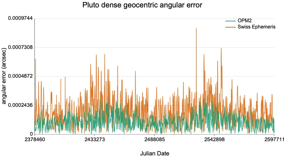
The dense geocentric angular-error validation output for the 600-year production instance is out/opm2-600y-selected-polished-swiss-geocentric-512.txt. The complete SVG curves are in out/opm2-600y-selected-polished-swiss-plots/angular/. The following thumbnails were generated by the same dense validation run using 512 Chebyshev nodes per segment plus endpoints.

Sun	Moon

Mercury	Venus

Mars	Jupiter

Saturn	Uranus

Neptune	Pluto

Appendix E. Native Residual Diagnostic Thumbnails

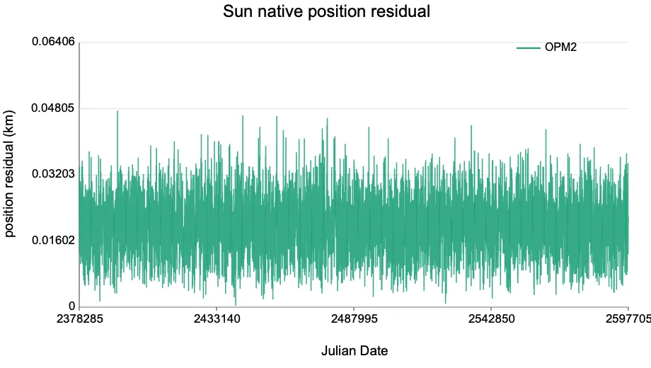
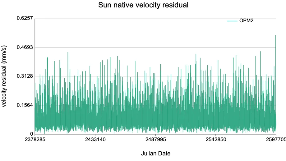
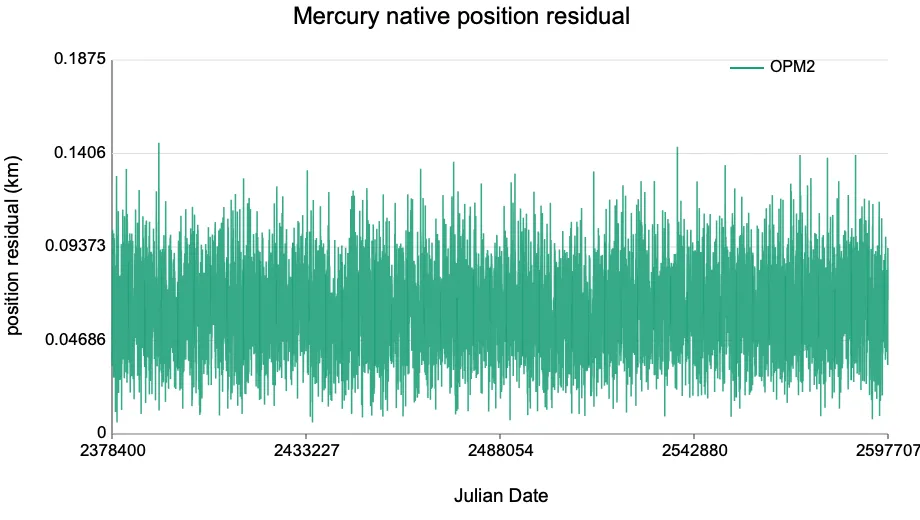
The native residual diagnostic output for the 600-year production instance is out/opm2-600y-selected-polished-native-residuals-512.txt. The complete SVG curves are in out/opm2-600y-selected-polished-native-plots/native/. The following thumbnails were generated by the same diagnostic run. Position residuals are in km and velocity residuals are in mm/s.

Sun position	Sun velocity

Mercury position	Mercury velocity

Venus position	Venus velocity

EMB position	EMB velocity

Moon position	Moon velocity

Mars position	Mars velocity

Jupiter position	Jupiter velocity

Saturn position	Saturn velocity

Uranus position	Uranus velocity

Neptune position	Neptune velocity

Pluto position	Pluto velocity

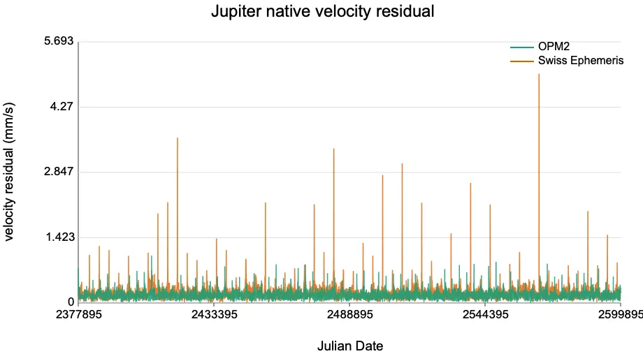
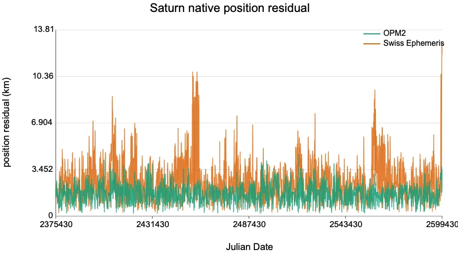
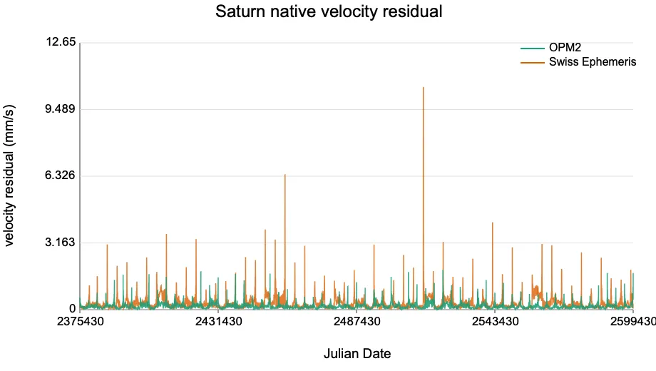
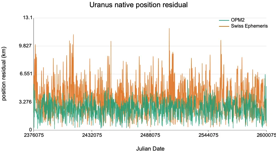
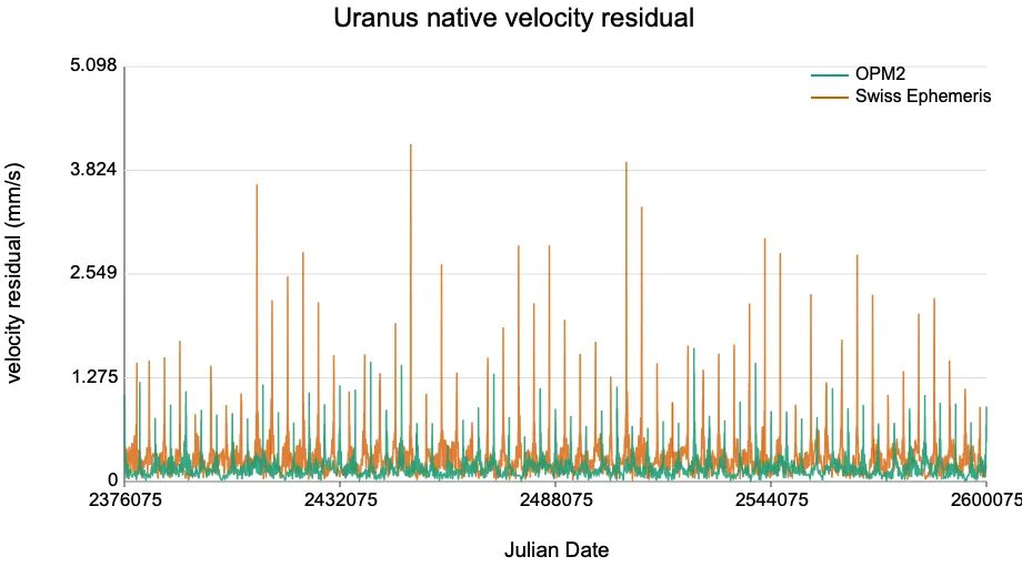
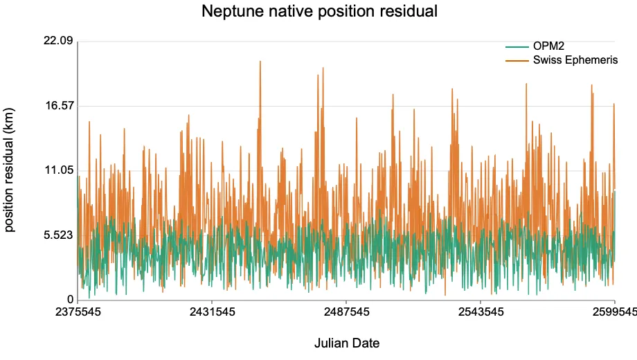
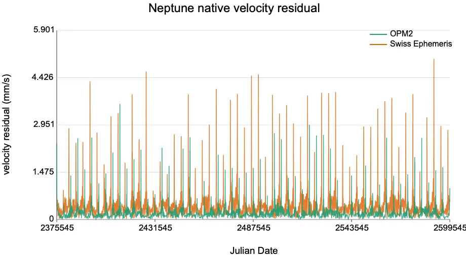
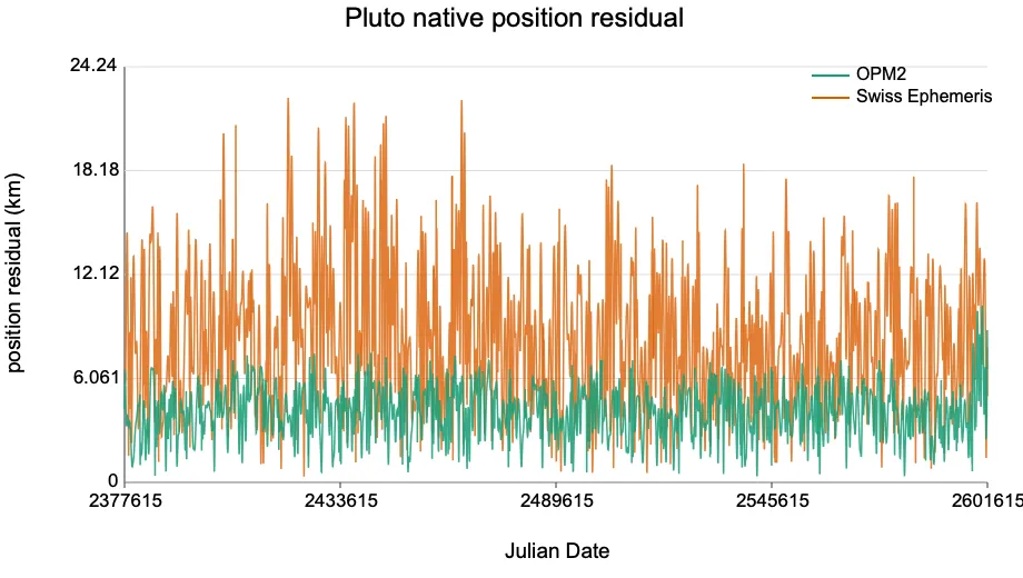
Appendix F. OPM vs Swiss Ephemeris Native Position/Velocity Residual Curves

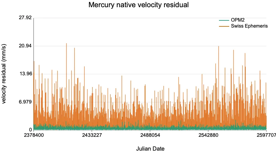
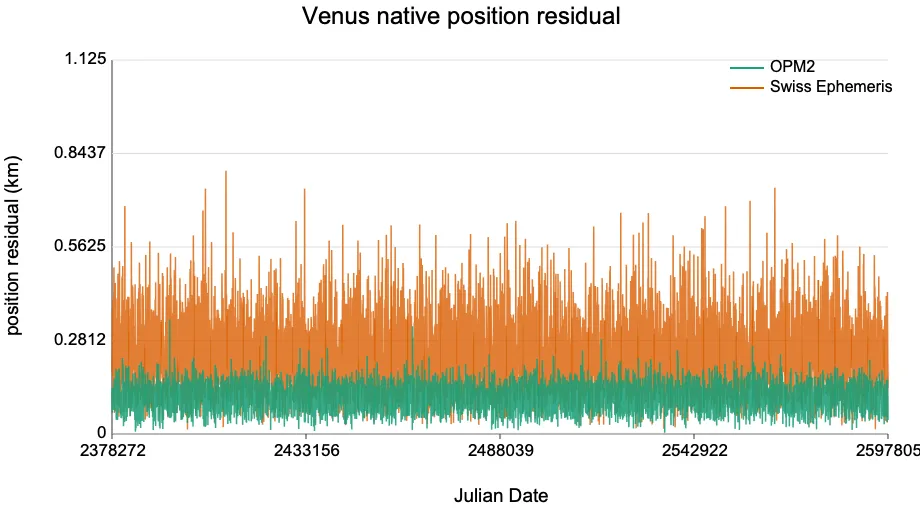
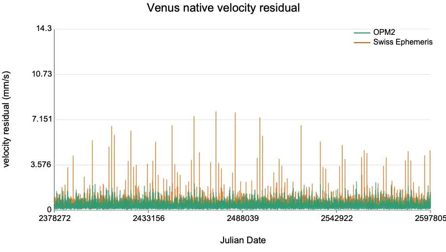
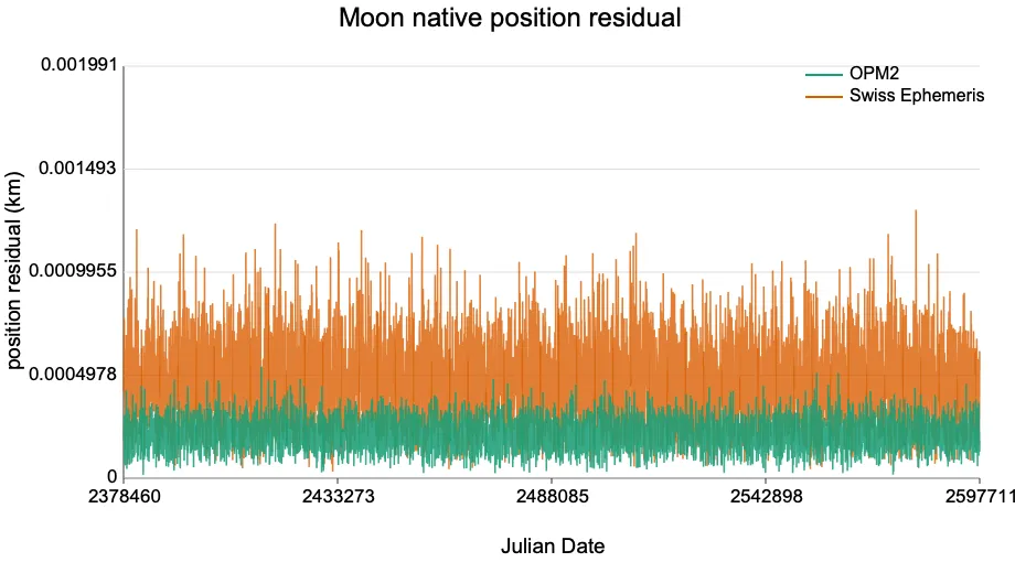
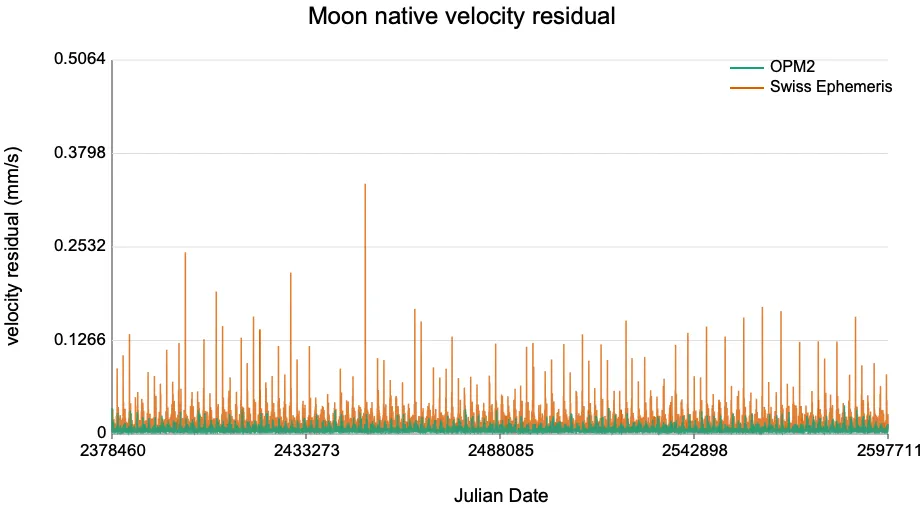
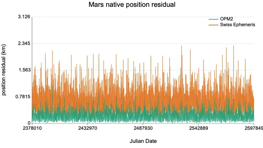
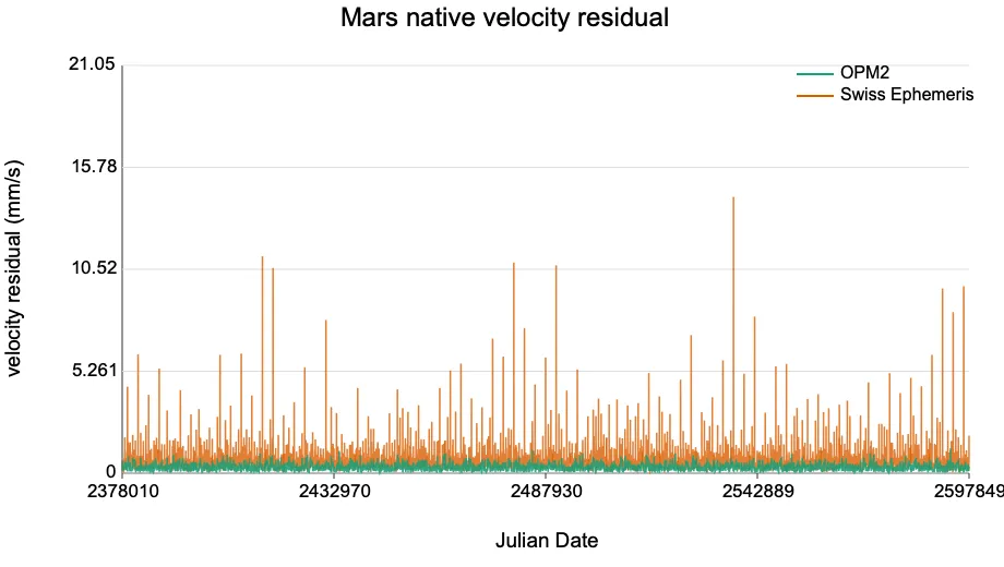
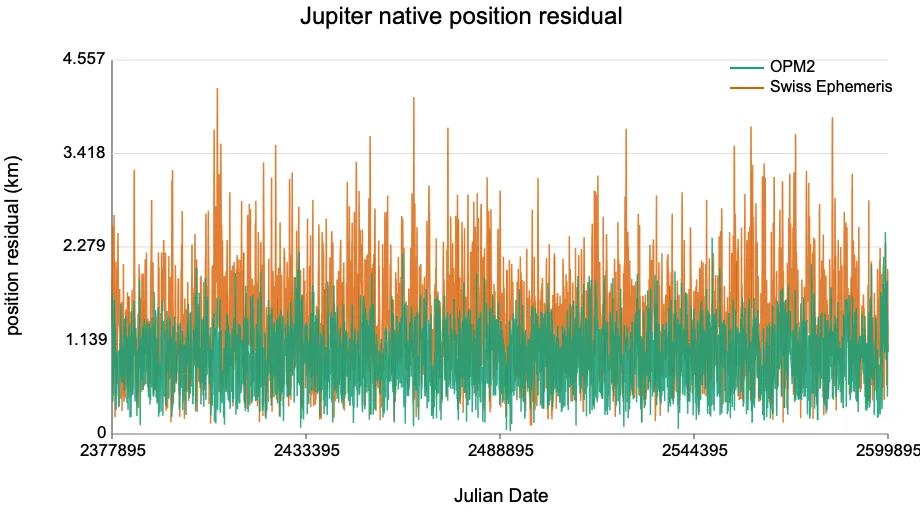
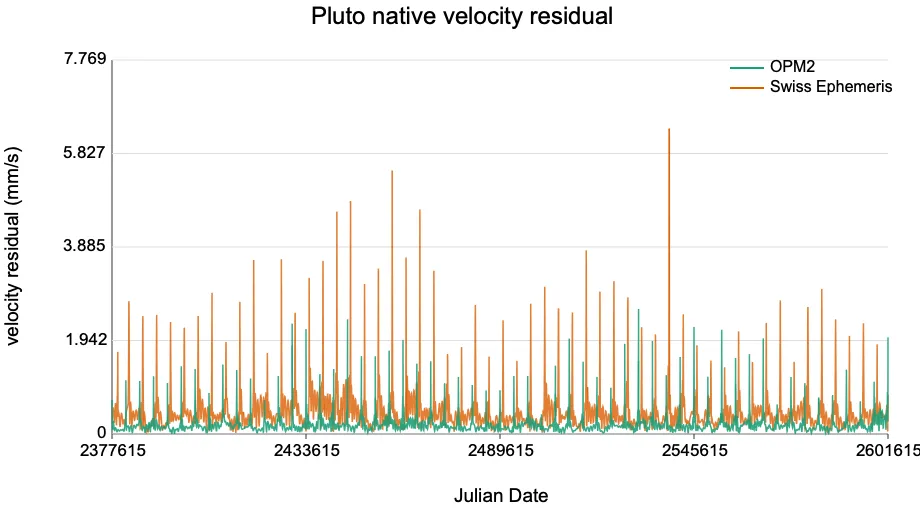
The OPM-vs-Swiss native-vector comparison data for the 600-year production instance come from out/opm2-600y-selected-polished-native-residuals-512.txt. The complete SVG curves are in out/opm2-600y-selected-polished-swiss-plots/native-opm-vs-swiss/. All curves use DE441 as truth. Green is OPM; orange is Swiss Ephemeris. Position residuals are in km and velocity residuals are in mm/s. The EMB Swiss native reference is synthesized from Earth SSB and the geocentric Moon vector in Table 3; the thumbnail section lists only the directly plotted Swiss-addressable bodies.

Sun position	Sun velocity

Mercury position	Mercury velocity

Venus position	Venus velocity

Moon position	Moon velocity

Mars position	Mars velocity

Jupiter position	Jupiter velocity

Saturn position	Saturn velocity

Uranus position	Uranus velocity

Neptune position	Neptune velocity

Pluto position	Pluto velocity

---